## YANIV ADD MAP (next year_)• 19. ANOVA assumptions
Motivating Scenario: You are ready to run an ANOVA to compare means among more than two groups. Before doing so, you need to check whether your data meet ANOVA’s assumptions (and know what to do if they do not).
Learning Goals: By the end of this subchapter, you should be able to:
List the assumptions of an ANOVA.
Evaluate if your data meet these assumptions.
Identify options for dealing with violations of these assumptions, and know how to choose among them.
The ANOVA shares a core set of assumptions with most standard linear models. The assumptions are:
Like the two-sample t-test, ANOVA assumes:
- Independence
- Random sampling (no bias)
- Equal variance among groups (homoscedasticity)
- Normality within each group, or more specifically, normality of each group’s sampling distribution.
Here we use the parviflora admixture data to look into these assumptions
ANOVA Assumes…
… Equal Variance Among Groups
Homoscedasticity means that the variance of residuals is independent of the predicted value. For our parviflora admixture proportions, we make only three predictions — one per population, so this essentially means we assume equal variance within each group. This makes sense, as we use a mean squares error in ANOVA. In fact, the very derivation of ANOVA assumes that all groups have equal variance.
As we can see the variance among groups differs quite substantially. So, we should think twice before conducting a standard ANOVA. Below I will introduce a Welch’s ANOVA, to accommodate this issue. But I will nonetheless analyze the data by a standard ANOVA as well to show you the mechanics. At the end we will compare and contrast results from a standard and Welch’s ANOVA to see how worried we should be about equal variance.
clarkia_hz|>
    group_by(site)|> # below I multiply the variance by a lot to make it easier to read.
summarise(var_admix_x_1e5 = var(admix_proportion) * 10000) |> kable(digits = 4)| site | var_admix_x_1e5 |
|---|---|
| SR | 0.0071 |
| S22 | 4.0221 |
| SM | 0.5128 |
| S6 | 1.6371 |
… Normal Residuals w.in Groups
As in the t, and in all linear models, we use the normal framework to evaluate the null hypothesis proposed by an ANOVA. Of course data are rarely perfectly normal, but the data we are examining here seem particularly far from this assumption (Figure 1.1). I will proceed here, not because this is the right thing to do, but simply to show you how an ANOVA works.
library(patchwork)
qq_clarkia_hz <- clarkia_hz|>
    ggplot(aes(sample = admix_proportion))+
    geom_qq()+
    geom_qq_line()+
    facet_wrap(~site, scales = "free_y", nrow = 1)

hist_clarkia_hz <- clarkia_hz|>
    ggplot(aes(x = admix_proportion))+
    geom_histogram( bins = 10, color = "white")+
    facet_wrap(~site, nrow = 1, scales = "free_y")

qq_clarkia_hz / hist_clarkia_hz + plot_annotation( tag_levels = "A" )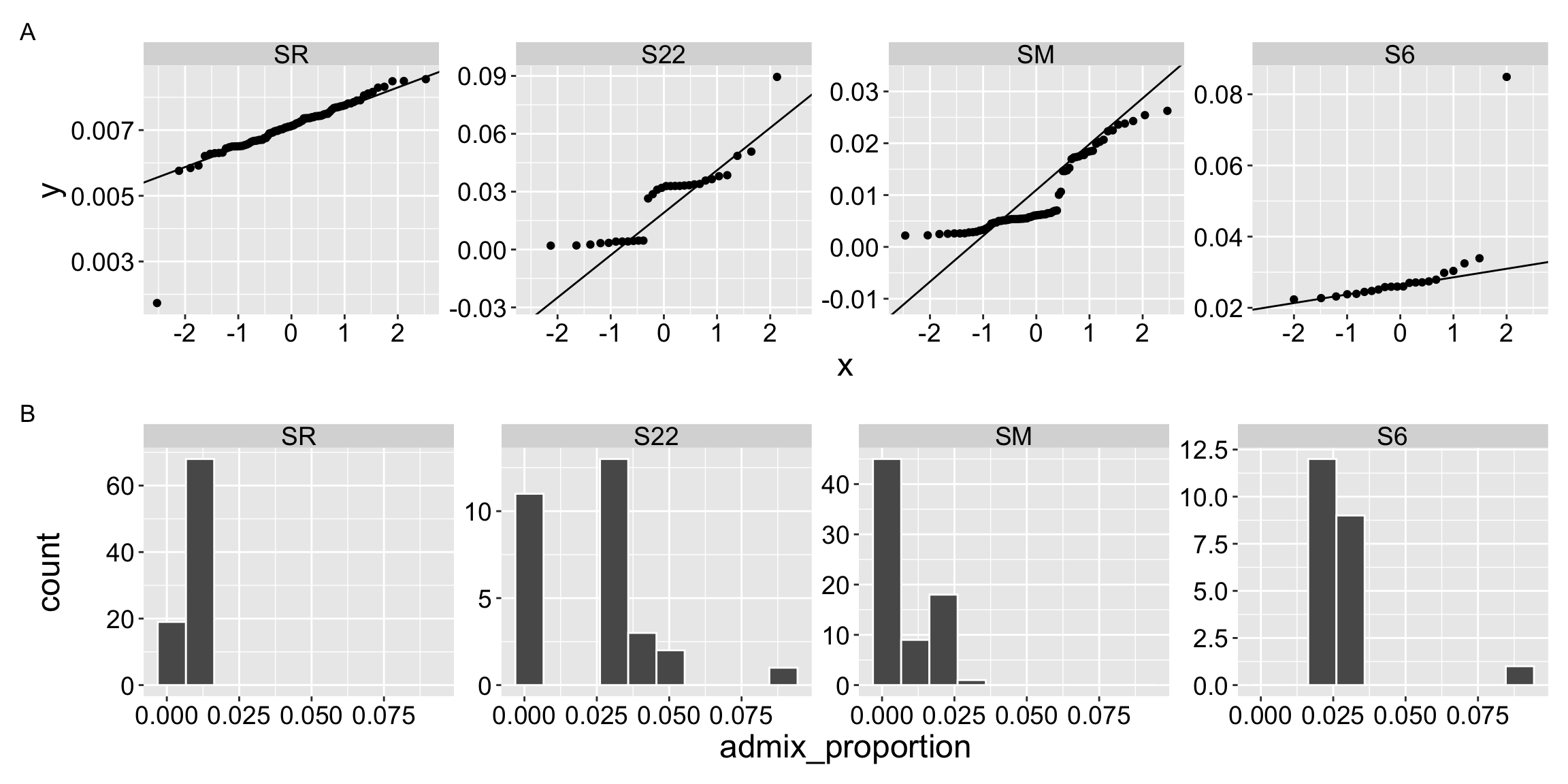
… Independence (w.in Groups)
Ugh the news gets even worse. These samples are taken from a reasonable proportion of the extant plants and have a spatial structure to them. My sense is that they are siblings or even genetically identical “clones”. The appropriate statistical procedure is not clear, but we will hold our nose, do our best, and acknowledge the potential non-independence.
… Unbiased Sampling (w.in Groups)

WOOT!!! NAILED IT We did a fantastic job sampling without bias. Believe me!
What to do when you violate assumptions
We’ll continue using these data to learn how ANOVA works. But when the assumptions are clearly broken, as in this example, we need to think about what to do. I wan to emphasize that there’s usually not a single right answer, and that your choice will be a compromise between trade-offs of each potential approach. Below are some options, along with my (strong) opinions. I also note that you don’t need to pick a single analysis, sometimes it makes sense to present results from different types of analyses to show that your take-home message is robust to any specific assumptions.
Most importantly, think about what you’re doing and why. While you should not run a statistical test that gives meaningless results, there’s usually a trade-off between statistical purity and clear communication of your results. So don’t rush to the most statistical pure approach if it means your results are difficult to interpret.
If you’re interested in NHST, breaking assumptions means that you p-values aren’t properly calibrated, so you cannot literally interpret your p-value. But how often do you care about the exact p-value? If you’re worried about misleading confidence intervals, consider the trade-offs between having these perfectly calibrated, and loss of information that may occur when presenting results on a scale that is difficult to interpret. Let clarity about your goals and the meaning of your results take precedence over strict rule following.
Minor violations: If the test is known to be robust to small deviations—like mild non-normality or modest differences in variance—you can usually proceed without concern.
Major non-normality: When data are far from normal within groups, consider transforming your data (e.g., log, square root) or using a model that explicitly captures the shape of the distribution that generated your data. We’ll return to this idea later when we discuss generalized linear models.
Robust approaches: Methods like Welch’s ANOVA (which allows group variances to differ, below), or approaches that “trim” extreme outliers, are generally solid and defensible choices.
Permutation tests: While tempting, permutation-based ANOVAs often introduce new violations - particularly non-independence and can make variance unequal between groups - so interpreting these results is difficult.
Rank-based tests: Alternatives like the Kruskal–Wallis test assess differences in medians rather than means and are less sensitive to assumption violations. However, their effect sizes are harder to interpret in practical or biological terms.
Welch’s ANOVA when variance differs
You can use a Welch’s ANOVA when variance differs substantially among groups. Welch’s ANOVA has the same underlying logic as a standard ANOVA, but gives more weight to groups whose means from samples with smaller variance. This means that F and the degrees of freedom etc can be interpreted similarly as in a standard ANOVA, but are calculated differently.
The oneway.test() function in R uses a Welch’s ANOVA by default:
oneway.test(admix_proportion ~ site, data = clarkia_hz)
    One-way analysis of means (not assuming equal variances)

data:  admix_proportion and site
F = 32.224, num df = 3.00, denom df = 52.34, p-value = 6.117e-12
Here, we resoundingly reject the null hypothesis that between-group variability equals within-group variability.