• 18. F and anova in R

Motivating Scenario: Now that you know what goes into calculating the sums of squares, degrees of freedom, mean squares, and F, you can want R to do this all for you. Here, we run an ANOVA in R and learn how to read the results it gives back.

Learning Goals: By the end of this subchapter, you should be able to:.

Run a one-way ANOVA in R using both aov() |> summary() and lm() |> anova() pipelines.
Interpret the ANOVA table which includes sums of squares, mean squares, F statistic, and p-value.
Use the broom package to:
- tidy() ANOVA results and
- glance() at model-level summaries (like \(R^2\)).

In the previous sections we worked through the math and the theory, and even how we could use R to do our calculations for us. This is all useful and I hope it helps you understand what is going on behind the scenes. But now that we know what’s going on, we can have R do our work for us. Here, I show you two ways to have R calculate F and conduct an anova test for us.

In so doing we consider how to interpret R’s output, and how to convert it to a “tidy” format with broom’s glance() and tidy() functions.

The `aov() |> summary()` pipeline

The aov() function is built specifically to conduct ANOVA in R. To do so, it uses the familiar formula syntax: (RESPONSE ~ EXPLANATORY, data = DATA)

admix_anova <- aov(admix_proportion ~ petal_color, data= clarkia_hz )

The aov() object contains the relevant sums of squares (which match our hand calculations!) and the degrees of freedom. To actually view the ANOVA table, we use summary() on the aov object. This table includes the sums of squares, mean squares, the F statistic, and the associated p-value.

summary(admix_anova)

            Df   Sum Sq   Mean Sq F value   Pr(>F)    
petal_color  1 0.001831 0.0018312   76.54 3.49e-11 ***
Residuals   44 0.001053 0.0000239                     
---
Signif. codes:  0 '***' 0.001 '**' 0.01 '*' 0.05 '.' 0.1 ' ' 1
27 observations deleted due to missingness

broom’s tidy() function provides this output in a “tidy” format, its glance() function shows some relevant summaries of the model (including \(R^2\)).

library(broom)
tidy(admix_anova)

# A tibble: 2 × 6
  term           df   sumsq    meansq statistic   p.value
  <chr>       <dbl>   <dbl>     <dbl>     <dbl>     <dbl>
1 petal_color     1 0.00183 0.00183        76.5  3.49e-11
2 Residuals      44 0.00105 0.0000239      NA   NA

glance(admix_anova)

# A tibble: 1 × 6
  logLik   AIC   BIC deviance  nobs r.squared
   <dbl> <dbl> <dbl>    <dbl> <int>     <dbl>
1   180. -355. -349.  0.00105    46     0.635

The `lm() |> anova()` pipeline

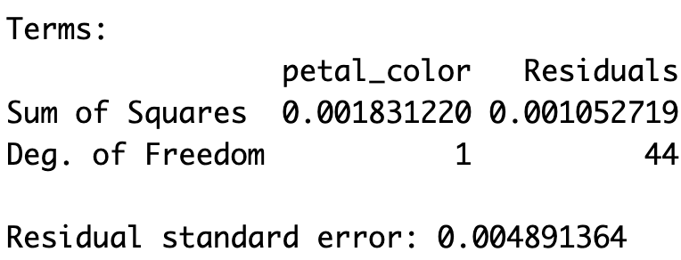
Alternatively, we can fit a linear model and then hand it to anova() to create the ANOVA table. This produces the same output as aov() |> summary(), but the intermediate object is an lm object rather than an aov object. Sometimes one format is just easier to work with than the other, but your results will be the same.

lm(admix_proportion ~ petal_color, data= clarkia_hz ) |>
  anova()

Analysis of Variance Table

Response: admix_proportion
            Df    Sum Sq    Mean Sq F value    Pr(>F)    
petal_color  1 0.0018312 0.00183122  76.539 3.486e-11 ***
Residuals   44 0.0010527 0.00002393                      
---
Signif. codes:  0 '***' 0.001 '**' 0.01 '*' 0.05 '.' 0.1 ' ' 1

If we want more information about our model, we can pass the lm object to glance():

lm(admix_proportion ~ petal_color, data= clarkia_hz ) |>
  glance()

# A tibble: 1 × 12
  r.squared adj.r.squared   sigma statistic  p.value    df logLik   AIC   BIC
      <dbl>         <dbl>   <dbl>     <dbl>    <dbl> <dbl>  <dbl> <dbl> <dbl>
1     0.635         0.627 0.00489      76.5 3.49e-11     1   180. -355. -349.
# ℹ 3 more variables: deviance <dbl>, df.residual <int>, nobs <int>

glance() works on model objects like lm or aov, but not on the ANOVA table itself. So lm() |> anova() |> glance() returns an empty tibble.

Here is a brief summary of common linear model workflows in R and what they give us.

Task	Function(s)	Output object
Run ANOVA directly	`aov() \|> summary()`	ANOVA table
Run via linear model	`lm() \|> anova()`	same ANOVA table, but model object is `lm`
Tidy results	`broom::tidy()`	tidy table of terms
Model summary	`broom::glance()`	includes R², df, etc.

The aov() |> summary() pipeline

The lm() |> anova() pipeline

The `aov() |> summary()` pipeline

The `lm() |> anova()` pipeline