• 11. Sampling

Motivating Scenario: We need to know about sampling to do statistics!

Learning Goals: By the end of this subsection, you should be able to:

Explain why sampling is a necessary and fundamental part of statistics.
Distinguish between a population parameter and a sample estimate.
Describe and differentiate between random, stratified random, and haphazard sampling methods.
Explain what to do when you cannot sample randomly, and how to be cautious about interpreting data from a non-random sample.

Estimate population parameters by sampling

Of course, if we already had a well characterized population, there would be no need to sample – we would just know actual parameters, and there would be no need to do statistics. It’s usually too much work, costs too much money, or takes too much time to characterize an entire population and calculate its parameters. So we take estimates from a sample of the population.

“Sampling” does not always mean taking a subsample from a larger population:

For example, in an experiment we interfere with a system and see how this intervention changes some outcome, or in flipping a coin we generate a new outcome that had not yet happened. Nonetheless, we can use the metaphor of sampling in all of these cases.

As such, being able to imagine the process of sampling – how we sample, what can go wrong in sampling is perhaps the most important part of being good at statistics. I recommend walking around and imagining sampling in your free time.

How to Sample

Random sampling is the gold-standard sampling design. In a truly random sample, every individual in a population has an equal chance of being selected. This can be achieved by giving each individual a unique number and then picking numbers from a random number generator (e.g., the sample() function in R).

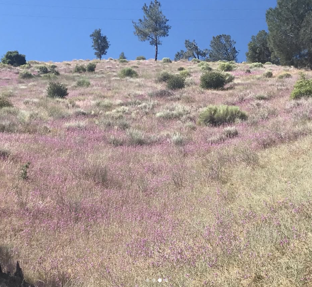
A wide shot of a sunny, grassy hillside sloping upwards. The hill is covered in a dense carpet of small pink wildflowers mixed with patches of tan, dry grass and larger green shrubs. A few tall, sparse trees are visible at the crest of the hill against a clear blue sky. — Figure 1: A California hillside covered in a dense bloom of pink Clarkia wildflowers, mixed with dry grasses and scattered shrubs under a clear blue sky. This vast, natural population illustrates a scenario where conducting a full census of every plant would be impractical, and truly random sampling would be quite challenging.

In practice, this can be difficult. It would take ages to number every Clarkia plant on a hillside with thousands of individuals (e.g. Figure 1). So, we often employ other sampling designs.

Stratified random sampling is a way to ensure that different subgroups within a population are represented. To do this, you first split the population into groups, or “strata” (e.g., plants on sunny vs. shady slopes), and then perform a random sample within each group.
Haphazard sampling (also called convenience sampling) is a non-random design. While not ideal, a haphazard approach with a clear, pre-defined plan can sometimes be sufficient. For example, you might decide to walk a transect line and sample the plant closest to the line every 10 meters.

SAMPLE RANDOMLY WHENEVER POSSIBLE!
If you cannot sample randomly, be explicit about your method. For example, our transect method is more likely to select plants in sparse areas than dense ones. Is that a problem? It depends on your question. If sampling is haphazard, you must critically consider and report how your method could introduce potential biases into your results.

Random sampling example

In the real world, taking a random sample from a population can be a challenge (see above). But in R this is very easy. I work through an example to better wrap our heads around sampling.

For this example, let us pretend that our hybrid zone data from SAW is a population (i.e. that we sampled every individual). I note this is for demonstration purposes only – if we had information for an entire population we would not sample. But this should help us think about sampling! We use the slice_sample() function, with the arguments being the tibble of interest, n the size of our sample. The output are the individuals we sampled!

Loading and formatting saw hybrid zone data.

hz_pheno_link <- "https://raw.githubusercontent.com/ybrandvain/datasets/refs/heads/master/clarkia_hz_phenotypes.csv"

saw_hz_pop <- read_csv(hz_pheno_link)|> 
  filter(site == "SAW") |>
  select(id,subspecies, node, protandry = avg_protandry, herkogamy = avg_herkogamy, petal_area = avg_petal_area)|>
  mutate(petal_area = round(petal_area, digits = 2))

sample_size <- 10

# make a sample 
saw_hz_sample <- saw_hz_pop|> 
 slice_sample(n=sample_size)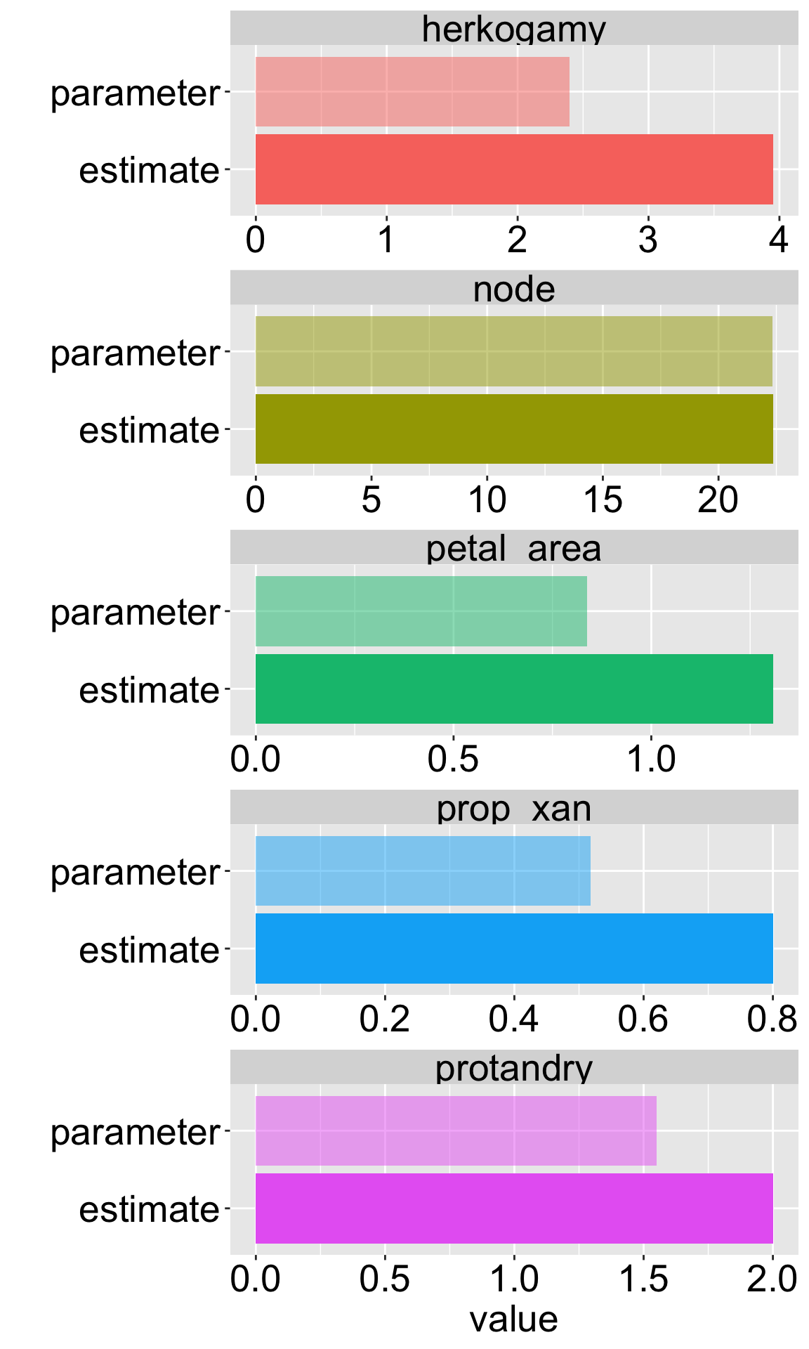

Figure 2: Comparing parameters from our ‘population’ to estimates from our ‘sample’ for numerous traits.

Parameters versus estimates

We can now compare our estimates from our sample of size ten to our “true” parameter (remember this is not our true parameter we are just pretending that our initial sample is the entire population so we can learn this stuff better).

Figure 2 clearly shows that our sample estimates differ from the true population parameters. This chance deviation is sampling error in action. While some estimates are close, others are not, highlighting the fundamental challenge for statisticians: how do we quantify our uncertainty about the true parameter when we only have one sample?

Code

long_estimate <- estimates |> mutate(measure = "estimate")|>pivot_longer(-measure)
long_param <- parameters |> mutate(measure = "parameter")|>pivot_longer(-measure)
bind_rows(long_estimate, long_param) |>
  rename(trait= name)|>
  ggplot(aes(y = measure, x = value, fill = trait, alpha = measure))+
  geom_col()+
  labs(y="")+
  facet_wrap(~trait, scales = "free_x",ncol = 1)+
  scale_alpha_discrete(range = c(1,.5))+
  theme(legend.position = "none",
        axis.text = element_text(size = 20),
        axis.title = element_text(size = 20),
        strip.text =  element_text(size = 20))