• 17. Two-t Calculations

Motivating scenario: We want to comparing means of two-samples, how do we summarize this difference?

Learning goals: By the end of this section, you should be able to:

• Calculate the common summaries of two samples.
  • Means.
  • “Pooled” variance.
    
  • Cohen’s D.
    

ril_link <- "https://raw.githubusercontent.com/ybrandvain/datasets/refs/heads/master/clarkia_rils.csv"
SR_rils <- readr::read_csv(ril_link) |>
  filter(location == "SR") |>
  select(ril, petal_color, mean_visits) |>
  filter(!is.na(mean_visits), !is.na(petal_color))

SR_rils  <- SR_rils                          |> 
  mutate(log_visits = log(.2 + mean_visits))

---

Estimates

library(ggforce)
ggplot(SR_rils, aes(x = petal_color,
                    y = log_visits,
                    fill = petal_color))+
  geom_sina(pch = 21, size = 7)+
  scale_fill_manual(values = c("pink", "white"))+
  stat_summary(fun.data   = "mean_cl_normal", linewidth = 3)+
  stat_summary(geom = "line", linewidth = 1, linetype = 2,aes(group = 1))+
  theme(legend.position = "none",
        axis.text  = element_text(size = 26),
        axis.title = element_text(size = 26))+
  labs(y = "log (0.2 + visits)")

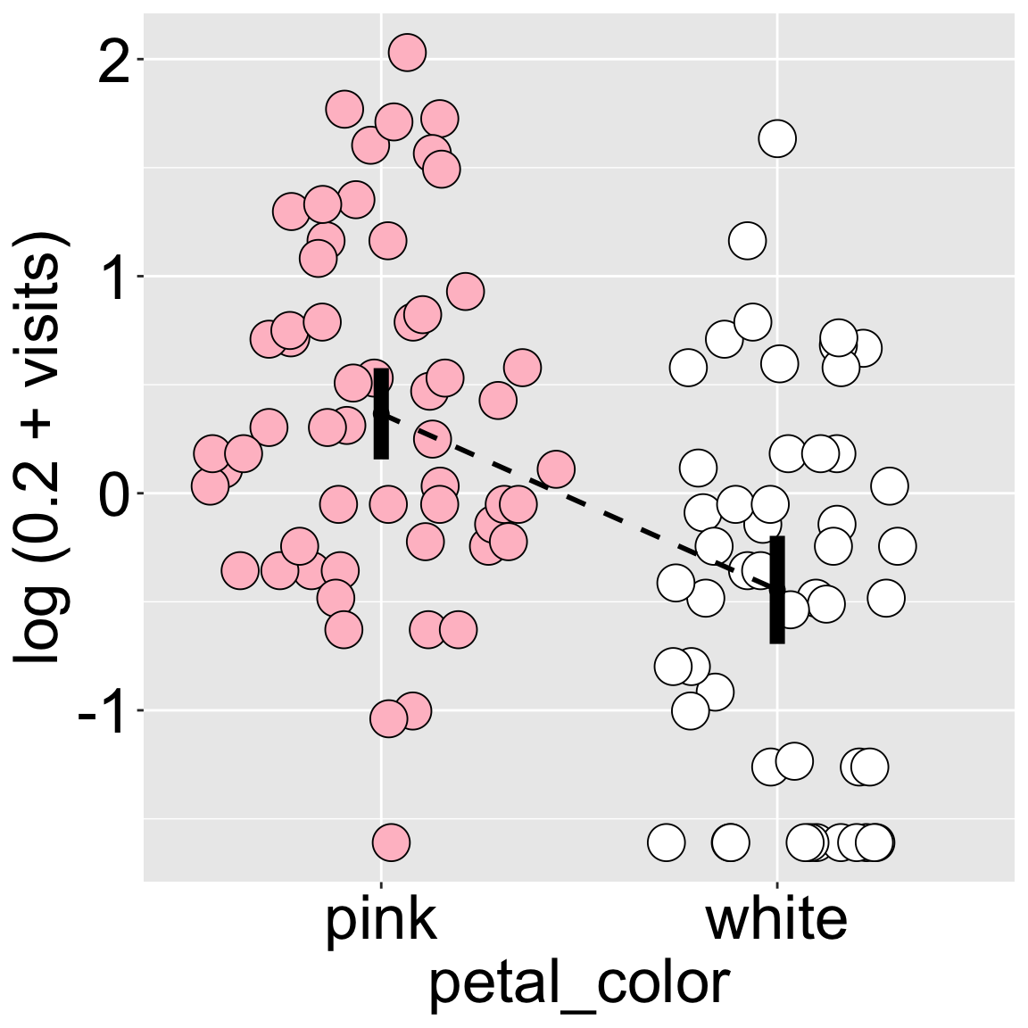
Figure 1: Each point shows an individual RIL’s mean pollinator visits on a log(visits + 0.2) scale. Flower colors means and 95% confidence intervals are plotted as thick black bars, with a dashed line connecting the group means for comparison.

Here’s a brief refresher of our previously introduced standard summaries of associations between a categorical explanatory variable and a continuous response.

Because we are calculating statistics on transformed data, we should summarise the transformed data. Later in this section we will learn how to back-transform.

Estimating summaries of each group:

We can summarise within group means, and variances (or even 95% CI if we want etc) as we saw in the previous chapter. (Some of) these high-level summaries are presented in Figure 1 and calculated below:

petal_color	MEAN	VAR	N
pink	0.366	0.627	57
white	-0.445	0.768	50

color_visit_summaries <- SR_rils |>
  group_by(petal_color)|>
  summarise(MEAN = mean(log_visits),
            VAR        = var(log_visits),
            N                 = n())

Estimating summaries of differences:

We would also like to summarise the data jointly, including the variance, the difference in groups means, and a standardized summary of this difference:

• The pooled variance: To both estimate the effect size as Cohen’s D, and estimate uncertainty we need to calculate the variance. But we have two groups, so we need something like “the average variance within each group.” The pooled variance, \(s^2_p\) – the variance in each group weighted by their degrees of freedom and divided by the total degrees of freedom is this average (see margin for hand calculation).

\[ \begin{align} s^2_p &= \frac{df_1 \times s^2_1 + df_2 \times s^2_2}{df_1+df_2} \\ &= \frac{df_\text{pink} \times s^2_\text{pink} + df_\text{white} \times s^2_\text{white}}{df_\text{pink}+df_\text{white}} \\ &= \frac{(57-1)\times 0.627 + (50-1)\times 0.768}{(57-1)+(50-1)} \\ &= 0.693 \end{align} \]

• The difference in means: To find this simply subtract one from the other: \(\text{mean}\_\text{diff}= 0.366 - (-0.455)= 0.811\).
  
  

• Cohen’s D as the difference in means weighted by the pooled standard deviation. Cohen’s D \(=\frac{\text{mean diff}}{s_p}\) \(=\frac{0.811}{\sqrt{0.693}}\) \(= 0.974\). This is a large effect size!!!

We can calculate these global summaries from summaries of each petal color (above):

summary	estimate
mean_diff	0.811
pooled_var	0.693
pooled_sd	0.832
cohens_D	0.975

color_visit_summaries|>
    summarise(mean_diff  = diff(MEAN) |> abs(), 
              pooled_var = sum((N-1)*(VAR)) / (sum(N)-2),
              pooled_sd  = sqrt(pooled_var),
              cohens_D   = mean_diff / pooled_sd)