Motivating scenario: We want to know if two binary things are associated. Here we show how to use permutation to test the null hypothesis of no such association.
Learning goals: By the end of this chapter you should be able to:
Calculate expected counts from a 2X2 table.
Calculate \(chi^2\) for such data and compare it to its null sampling distribution to find a p-value.
Interpret the result of this test.
We are often interested to know if two variables are associated. The \(\chi^2\) statistic is useful when examining associations between two categorical variables. For example, we can calculate a deviation from expected counts to see if pink-flowered parviflora RILs are more likely to receive a pollinator than are white-flowered parviflora RILs.
Quantifying associations
As you may recall, if two categorical outcomes are independent, the probability of both occurring together equals the product of their individual probabilities. For example, if these two variables are independent, we would expect the probability that a plant is both pink-flowered and visited by a pollinator to equal the proportion of pink flowers multiplied by the proportion of flowers receiving a pollinator visit. We can quantify the association between two binary variables as:
The covariance: \(Cov_{A,B} = P_{AB} -P_A \times P_B\).
The correlation: \(r_{A,B}=\frac{Cov_{A,B}}{s_A,s_B}\).
This formula is approximately right, but to get the answer exactly we would need to introduce Bessel’s correction (i.e. the denominator should be \(n-1\), not \(n\)). For now, this is good enough.
This formula is approximately correct, but to get the exact value we’d need to include Bessel’s correction—that is, divide by n – 1 instead of n (we could achieve this by multiplying by \(n /(n-1)\). For our purposes, this simpler version is good enough to capture the idea.
So, for our example, the covariance between pink flowers and receiving a pollinator visit among parviflora RILs at site Sawmill Road is 0.0502, and the correlation is 0.310.
This bootstrap-based 95% confidence interval does not cross zero, suggesting that we should reject the null hypothesis of no association.
To formally evaluate this idea using null hypothesis significance testing (NHST), we need:
A test statistic to measure,
A way to generate the sampling distribution of this test statistic under the null hypothesis of no association.
As you can see by permutation, using our observed correlation as the test statistic, this suggestion is correct. More precisely, we find a p-value of 0.0027. We therefore reject the null hypothesis.
Everything above is 100% legit. We can conduct a permutation test on any test statistic. However, as a bridge to the idea of an analytically derived null distribution, let’s calculate a \(\chi^2\) value as our test statistic:
Note that while \(\chi^2\) is a useful test statistic, it does not convey effect size, so it should be used for hypothesis testing rather than as a summary measure.
OBSERVATIONS
To start, we need the observed counts in each category:
We then need the expected counts in each category under the null of no expected association. To do so we multiply probabilities of each outcome to find the expected proportion in each category (same intuition above), and multiply by n to turn these expected proportions into expected counts:
sr_rils|>filter(!is.na(petal_color), !is.na(visited))|>summarise(n =n(), p_visited =mean(visited),p_pink =mean(petal_color=="pink"),pink_visit_expect = n * p_visited * p_pink,white_visit_expect = n * p_visited * (1-p_pink),pink_novisit_expect = n * (1-p_visited) * p_pink,white_novisit_expect = n * (1-p_visited) * (1-p_pink)) |>kable()
We can permute with the infer() pipeline. Note that we specify stat = "Chisq", and correct = FALSE. This later argument calcualtes the actual \(\chi^2\) value.
### permute the data 10k timesall_perms <- sr_rils|>specify(visited ~ petal_color,success ="TRUE") |>hypothesize(null ="independence") |>generate(reps =10000, type ="permute") |>calculate(stat ="Chisq", correct =FALSE)
Plot the permutation results
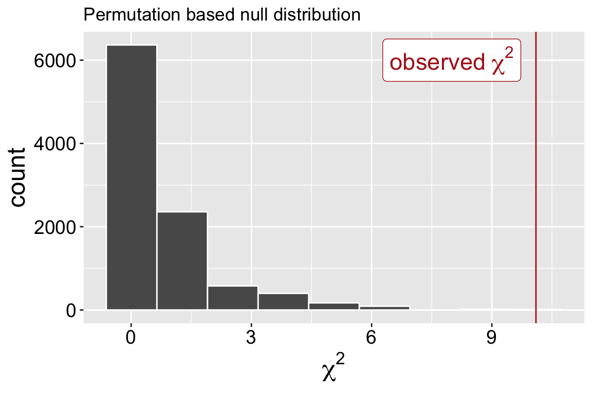
all_perms |>ggplot(aes(x = stat))+geom_histogram(bins =9, color ="white")+geom_vline(xintercept =10.1, color ="firebrick")+annotate(x =8,y =6000,color ="firebrick", geom ="label", label ="observed~chi^2", parse =TRUE, size =6)+labs(x =expression(chi^2), title ="Permutation based null distribution")
Figure 1: Permutation-based null distribution of χ² values under the hypothesis of independence. The red vertical line marks the observed χ² statistic from the real petal color and pollinator visitation data at the Sawmill Road site.
We can use this to find the p-value. Note that we only examine the right tail of the \(\chi^2\) distribution because it encompasses all possible ways to deviate from expectations. This analysis confirms our rejection of the null. It appears that pink flowers are more likely to receive pollinator visits than white flowers.
# calculate the actual chi2observed_chi2 <- sr_rils|>specify(visited ~ petal_color,success ="TRUE") |>hypothesize(null ="independence") |>calculate(stat ="Chisq", correct =FALSE)get_p_value(obs_stat = observed_chi2, all_perms, direction ="right" )