18. F this!
Motivating scenario: you have a fresh new data set and want to check it out. How do you go about looking into it?
Learning goals: By the end of this chapter you should be able to
- Explain how total variability can be partitioned into model (explained) and residual (unexplained) components, and interpret visual representations of this partitioning.
- Calculate and interpret key values in an ANOVA analysis including:
- Mean squares for the model and error terms.
- The F statistic as theratio of mean squares.
- \(R^2\) as a measure of effect size in one-way models.
- Mean squares for the model and error terms.
- Recognize the connection between the two sample t test and the F test when comparing two groups.
- Recognize the assumptions of ANOVA and interpret correlations with care.

In this chapter, we focus on the simplest case, comparing two groups, to better undertand what the F statistic represents (or What the \(f\) is going on!) We’ll connect this to concepts you already know (t-tests, sampling distributions), work through the math of partitioning variance, learn how to run ANOVA in R, and end by showing how these methods are all part of a unified linear model framework
The utility of \(F\)
In the coming chapters you will see that this view of “partitioning variance” has broad utility. In addition to its utility in partitioning variability within and among two groups, the approach in this chapter can be applied to
- More than two groups.
- A numeric explanatory variable.
- Multiple explanatory variables, and even
- Explanatory variables whose interaction influences the response variable.
We will work through these applications in coming chapters!
Data and hypotheses for this section
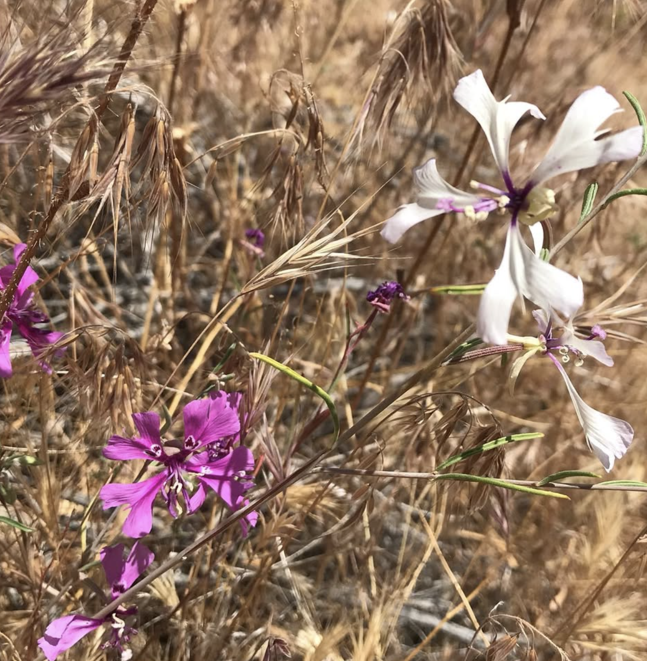
In the previous section, we saw that at Sawmill Road, pink parviflora RILs attracted more pollinators than did white parviflora RILs. We cared about this because we want to know if petal color influences hybridization – a question we will address later.
But there is a bigger motivating question than what happens in an experiment. That is, we want to know what has actually happened (and what is happening) in nature. In this chapter we get at the question of “does petal color influence hybridization?” in a somewhat backwards way. Instead of asking if pink flowers set more hybrid seed than white flowers, we analyze sequence data from pink and white flowered parviflora found in natural hybrid zones and ask if one petal color is associated with more introgression of xantiana ancestry.
Introgression is the incorporation of ancestry from one lineage into the genome of another, this happens by hybridization and subsequent backcrossing.
What’s ahead
In this section
We go through the mathemagical foundation of partitioning variance and how this relates to our understanding populations, and samples as draws from the sampling distribution.
We then show how to calculate the sum of squares error and sums of squares model and related measures.
Next, we introduce \(r^2\) as the “effect size” in such a model, and provide guidance on how to interpret this common summary.
We then show how to use this partitioning of variance to test the null hypothesis that all groups represent samples from the same population.
Before the chapter summary, we reflect a bit on correlation, causation and artifacts that may influence the patterns that we observe.
