lm(admix_proportion ~ site, data = clarkia_hz)|>
summary()• 19. Post hoc tests
Motivating Scenario:You rejected ANOVA’s null hypothesis that all group means are equal, but you’re still not happy. You want to know which groups differ!
Learning Goals: By the end of this subchapter, you should be able to:
- Distinguish between planned and unplanned (post hoc) comparisons.
- Conduct and interpret post hoc tests in R using functions such as
TukeyHSD(),glht(), andgames_howell_test(). - Interpret the results of pairwise comparisons and summarize which groups differ significantly.
- Avoid conducting post-hoc tests when you fail to reject ANOVA’s null hypothesis.
Motivation
ANOVA tells us that at least one group differs, but not which one. So, if you failed to reject the null, you’re done! But, if you did reject the null, this rejection might feel a bit hollow. You know that not all groups are the same, but you don’t know which groups differ from one another, so what’s the point even?
Here, we introduce post-hoc tests. Post hoc is Latin for “after this”. So, after you reject the null hypothesis that all groups come from the same population, you can run a post hoc test to see which groups differ from one another. Post hoc tests are much like pairwise t-tests, with slight modifications to control for false positives from multiple comparisons and to account for the fact that we’ve already rejected the overall null hypothesis that all groups are the same.
Do not run a post-hoc test if you fail to reject the null!
P-values from lm() |> summary() are wrong
You might think “Hey, I know how to find p-values associated with specific categories, I can just pipe the lm() output into summary().” But you would be wrong.
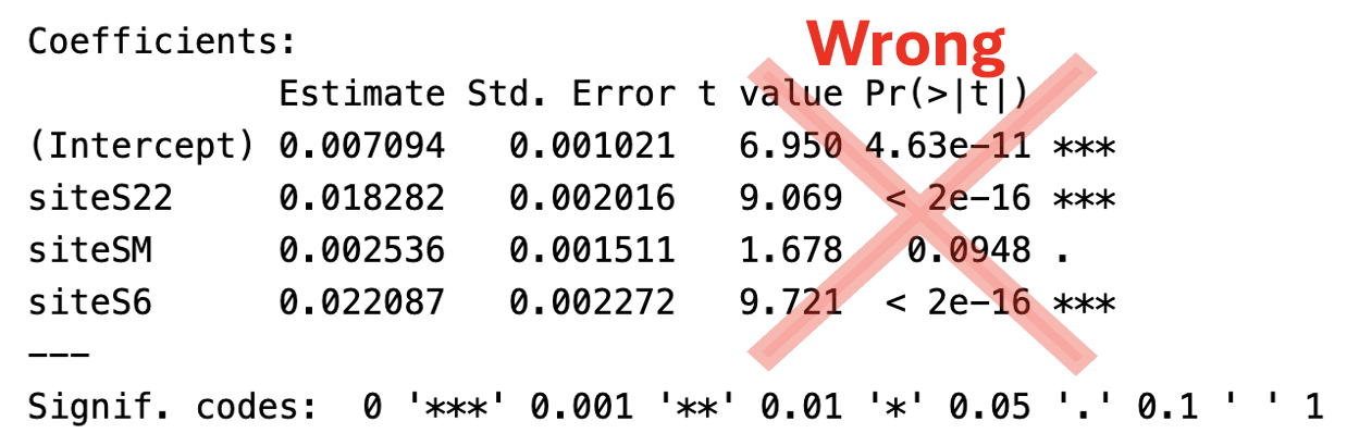
The outputs of this pipeline below is not fully meaningless, but are often misleading and should be ignored for multi-group comparisons. Hopefully the rows are familiar by now:
- Estimate: The estimated coefficient for that term in the model. For
(Intercept), it’s the mean of the reference group. For the other groups its the deviation from this mean.
- Std. Error: Is the uncertainty in this estimated value.
- t-value: Is the distance between our estimated value and 0 in units of standard errors (i.e.
Estimate / Std. Error).
- Pr(>|t|): Is the p-value:
2 * pt(abs(t), df, lower.tail = FALSE).
The estimate and standard error are usually interesting and meaningful. However, the t-value and p-value from the lm() |> summary() pipeline are usually useless and confusing.
For the
(Intercept)row, these relate to the null hypothesis that this value equals zero. In our case this is clearly stupid – the admixture proportion cannot be negative, so any nonzero value means we know the mean is not zero.the t- and p-values test whether each category differs from the reference level. While these hypotheses may be interesting, these summaries should still be ignored because:
- The t-value is wrong because it uses the total error degrees of freedom. This is wrong because in ANOVA, we partition variance among groups, so the residual df used here aren’t appropriate for multiple comparisons.
- The p-value is wrong because it comes from a wrong t-value, and because it does not acknowledge the multiple comparisons or the fact that we already reject the null from the ANOVA.
Additionally, this output does not allow us to test differences between two non-reference categories.
Post-hoc tests
There are two flavors of post-hoc tests.
In “planned comparisons” we are only interested in a small subset of the potential pairwise comparisons. In these cases, we limit our analysis to specific differences that are interesting for biological reasons, and ignore most of the potential comparisons. Planned comparisons provide more power, because we limit our attention to a small number of tests.
I will not focus planned comparisons. See this resource for more information.
In “unplanned comparisons” we are interested in all potential pairwise differences. Post-hoc test overcome the multiple comparisons problem by building a sampling distribution that conditions on there being at least one difference and numerous pairwise tests. Below we introduce numerous ways how to conduct unplanned post-hoc tests in R.
The Tukey-Kramer method’s is one common post hoc test. Its test statistic. \(q\) measures the distance bewtween group means in standard error units.
\(q= \frac{Y_i-Y_j}{SE}\), where \(\text{SE} = \sqrt{\text{MS}_\text{error}(\frac{1}{n_i}+ \frac{1}{n_j})}\).
From aov()
If we built our ANOVA with the aov() function, piping this output to the TukeyHSD() conducts this post-hoc test for you. You can see from the example below that we resoundingly reject the null that means are equal for all pairwise comparisons except SR vs SM, and S6 vs S22.
aov(admix_proportion ~ site, data = clarkia_hz)|>
TukeyHSD()| comparison | diff | lwr | upr | p.adj |
|---|---|---|---|---|
| S22-SR | 0.0183 | 0.0131 | 0.0235 | 0.0000 |
| SM-SR | 0.0025 | -0.0014 | 0.0064 | 0.3378 |
| S6-SR | 0.0221 | 0.0162 | 0.0280 | 0.0000 |
| SM-S22 | -0.0157 | -0.0211 | -0.0104 | 0.0000 |
| S6-S22 | 0.0038 | -0.0031 | 0.0107 | 0.4859 |
| S6-SM | 0.0196 | 0.0136 | 0.0255 | 0.0000 |
From lm()
If we built our anova as a linear model we can conduct a similar post-hoc test the glht() function in the multicomp package. This implementation of the Tukey test is slightly different from how it’s done in TukeyHSD(), so our p-values are slightly different.
We will see later that this approach can be generalized to more complex linear models.
library(multcomp)
lm(admix_proportion ~ site, data = clarkia_hz)|>
    glht(linfct = mcp(site = "Tukey"))|>
    summary()
     Simultaneous Tests for General Linear Hypotheses

Multiple Comparisons of Means: Tukey Contrasts


Fit: lm(formula = admix_proportion ~ site, data = clarkia_hz)

Linear Hypotheses:
               Estimate Std. Error t value Pr(>|t|)
S22 - SR == 0  0.018282   0.002016   9.069  <0.0001 ***
SM - SR == 0   0.002536   0.001511   1.678    0.329
S6 - SR == 0   0.022087   0.002272   9.721  <0.0001 ***
SM - S22 == 0 -0.015746   0.002065  -7.626  <0.0001 ***
S6 - S22 == 0  0.003805   0.002672   1.424    0.477
S6 - SM == 0   0.019551   0.002316   8.443  <0.0001 ***
---
Signif. codes:  0 '***' 0.001 '**' 0.01 '*' 0.05 '.' 0.1 ' ' 1
(Adjusted p values reported -- single-step method)
From Welch’s ANOVA
The Games Howell test, available in the rstatix package (as games_howell_test()), is a post-hoc test which does not assume equal variance among groups. You can see that our main conclusions hold, but that we have slightly more power and can now reject the null that SR and SM have the same admixture proportion.
However I worry that this power is unearned, as a I fear the low variance in sites SR and SM may reflect non-independence of data at each site.
library(rstatix)
games_howell_test(admix_proportion ~ site, data = clarkia_hz)| .y. | group1 | group2 | estimate | conf.low | conf.high | p.adj | p.adj.signif |
|---|---|---|---|---|---|---|---|
| admix_proportion | SR | S22 | 0.0183 | 0.0083 | 0.0283 | 0.0001 | *** |
| admix_proportion | SR | SM | 0.0025 | 0.0003 | 0.0048 | 0.0180 | * |
| admix_proportion | SR | S6 | 0.0221 | 0.0145 | 0.0297 | 0.0000 | **** |
| admix_proportion | S22 | SM | -0.0157 | -0.0259 | -0.0056 | 0.0010 | *** |
| admix_proportion | S22 | S6 | 0.0038 | -0.0083 | 0.0159 | 0.8380 | ns |
| admix_proportion | SM | S6 | 0.0196 | 0.0117 | 0.0274 | 0.0000 | **** |