• 16. Data summaries for t

Motivating scenario: You have some data of a single numeric variable. Before running any formal tests, you need to get to visualize and summarize the data!

Learning goals: By the end of this section, you should be able to:

Calculate the mean and standard deviation for a sample in R.
Define, calculate, and interpret Cohen’s D as a standardized measure of effect size for a one-sample test.
Create a histogram using ggplot2 to visualize the distribution of a sample.
Use summary statistics and a histogram to provide a preliminary, descriptive answer to a research question.

Code to load and process data

library(tidyr)
library(dplyr)
range_shift_file <- "https://whitlockschluter3e.zoology.ubc.ca/Data/chapter11/chap11q01RangeShiftsWithClimateChange.csv"
range_shift <- read_csv(range_shift_file) |>
  mutate(uphill = elevationalRangeShift > 0)|>
  separate(taxonAndLocation, into = c("taxon", "location"), sep = "_")

We have previously considered standard summaries of univariate data. Because the \(t\)-distribution assumes a normal distribution, we focus on standard parametric estimates. These include:

The mean: A measure of central tendency, \(\bar{x} = \frac{\Sigma x_i}{n}\).
The standard deviation: A measure of central spread, \(s = \frac{\Sigma(x_1-\bar{x})^2}{n-1}\).
Cohen’s D: A standardized measure of effect size, \(D = \frac{\bar{x}-\mu_0}{s}\).

We introduced Cohen’s D in the associations section, but can be used for a single numeric variable as well!

I calculate these below:

Summarizing range shift data
mean	sd	cohens_d
39.33	30.66	1.28

# set null to zero
mu_0 <-0 

# summarize data
range_shift_summary <- range_shift |>
  summarise(mean     = mean(elevationalRangeShift),
            sd       = sd(elevationalRangeShift),
            cohens_d = (mean - mu_0) / sd)

As a reminder

Cohen’s D between 0.50 and 0.80 is considered a “medium” effect.
Cohen’s D between 0.80 and 1.20 is considered a “large” effect.
Cohen’s D between 1.20 and 2.00 is considered a “very large” effect.

So, our observed Cohen’s D of 1.28 means that this effect is quite strong!

Data visualization

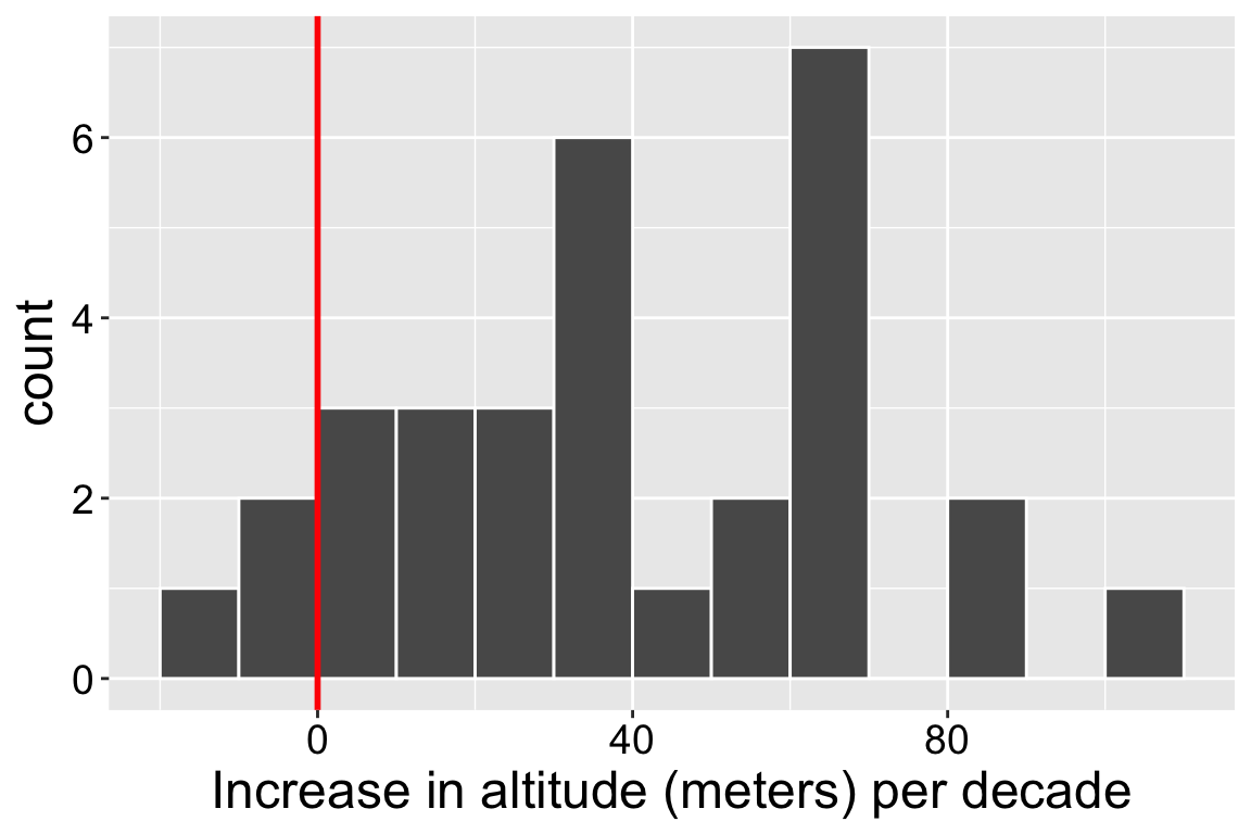
We will develop a few visualizations of our data. For now, I present a simple histogram. Figure 1, clearly shows that most species have moved uphill. It also allows us to evaluate if the data are normalish, as assumed by the t distribution. We spend the next section thinking harder about assumptions of the t distribution, and if our data.

Code to make our histogram

range_shift |>
 ggplot(aes(x = elevationalRangeShift ))+
 geom_histogram(color = "white",
                breaks = seq(-20,110,10))+
  geom_vline(color = "red", lty = 2, xintercept = 0)+
  labs(x = "Per decade increase in altitude (meters).")

A histogram of elevational range shifts. The x-axis ranges from roughly -20 to 100, and the y-axis (count) goes up to 7. Most of the bars are to the right of a vertical red line at x=0, indicating that most species groups shifted to higher elevations. — Figure 1: A histogram showing the distribution of observed elevational range shifts (in meters per decade) for 30 taxonomic groups. The vertical red line indicates a shift of zero, the value specified by the null hypothesis. Data from Chen et al. (2011).