• 14. The frogs – Applied Biostatistics

Case study: Mate choice & fitness in frogs

There are plenty of reasons to choose your partner carefully. In much of the biological world a key reason is “evolutionary fitness” – presumably organisms evolve to choose mates that will help them make more (or healthier) children. This could, for example explain Kermit’s resistance in one of the more complex love stories of our time, as frogs and pigs are unlikely to make healthy children.

In fact they will form fewer hybrids by mating than will parviflora and xantiana.

To evaluate this this idea Swierk & Langkilde (2019), identified a males top choice out of two female wood frogs and then had them mate with the preferred or nonpreferred female and counted the number of hatched eggs. The raw data are available here

A wood frog with a brown and tan patterned body, sitting on a white background. The frog has a distinctive dark eye mask and slightly raised ridges along its back. — Figure 1: A picture of the woodfrog. Image contributed to wikipedia under a CC BY 2.0 license by Brian Gratwicke.

Concept check

Is this an experimental or observational study?

Experimental Observational

It’s an experimental study because the researchers actively intervened and manipulated a variable. They assigned males to mate with either a preferred or a non-preferred female, rather than just observing which mates they chose on their own.

Which of the following describes the biological hypothesis?

That males who mate with their preferred female will have higher fitness (more hatched eggs). That frogs and pigs cannot produce healthy offspring. That mate preference does not affect the number of hatched eggs. That there will be a difference in the number of hatched eggs between the two groups.

The core biological idea is that mate choice should be adaptive. Therefore, the hypothesis is that a male’s choice should lead to a better evolutionary outcome, in this case, higher reproductive success measured by the number of hatched eggs.

Why not “That there will be a difference in the number of hatched eggs between the two groups”? A biological hypothesis is based on a theory, and therefore predicts a specific direction, such as higher fitness from mate choice. The statement “that there will be a difference” is a non-directional statistical hypothesis; it lacks the underlying biological reasoning and direction.

What is the statistical null hypothesis (\(H_0\))?

The observed difference in mean hatched eggs in our sample is zero. Males who mate with preferred females will have more hatched eggs. The average number of hatched eggs between the two treatment groups does not differ. The study design is biased.

The null hypothesis (\(H_0\)) is the hypothesis of ‘no effect.’ It posits that there is no true difference in the average number of hatched eggs between the preferred and non-preferred groups in the population. Any difference we see in our sample is assumed to be due to random sampling variation.

Why not “The observed difference in mean hatched eggs in our sample is zero.”? Because null hypotheses are about population parameters not observed sample estimates.

Which of the following is a potential source of bias in this experiment?

If the 'non-preferred' females were systematically smaller or less healthy than the 'preferred' females. The study was only conducted on wood frogs. The frogs were collected from different ponds. Some matings might not produce any eggs.

Bias occurs when there is a systematic difference between your treatment groups that is not the treatment itself. If the non-preferred females were also different in another key aspect (like health or size), we wouldn’t be able to tell if the results were due to ‘preference’ or that other factor. Random assignment helps to prevent this.

Visualize Patterns

Loading, formating, and plotting the data

frogs <- read_csv("https://raw.githubusercontent.com/ybrandvain/biostat/master/data/Swierk_Langkilde_BEHECO_1.csv")|>
  dplyr::select(year, pond, treatment,hatched.eggs, total.eggs, num.metamorphosed,field.survival.num)%>%
  mutate_at(.vars = c("hatched.eggs", "total.eggs", "num.metamorphosed" , "field.survival.num"), as.numeric)
library(ggforce)
ggplot(frogs, aes(x = treatment, y = hatched.eggs, color = treatment, shape = treatment)) +
  geom_violin(show.legend = FALSE)+
  geom_sina(show.legend = FALSE, size = 6, alpha = .6) +  # if you don't have ggforce, use geom_jitter
  stat_summary(fun.data = mean_cl_boot, geom = "pointrange", color = "black", show.legend = FALSE,linewidth = 1.2)+
  theme(axis.title = element_text(size = 30),
        axis.text = element_text(size = 30))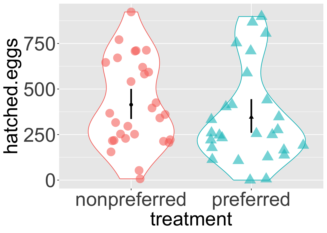

A violin plot comparing the number of hatched eggs between two treatments: non-preferred and preferred mates. The x-axis shows the treatment groups, and the y-axis represents the number of hatched eggs. The left violin, outlined in red with circular data points, represents the non-preferred treatment, while the right violin, outlined in blue with triangular data points, represents the preferred treatment. The black dot and error bars in the center of each violin plot represent the mean and standard error for each group. The non-preferred group shows a slightly wider distribution, with the mean closer to 500 hatched eggs, while the preferred group has a slightly narrower distribution, also centered around 500 hatched eggs. — Figure 2: Visualizing the frog mating data.

One of the first things we do with a new dataset is visualize it! A quick exploratory plot (refer back to our Intro to ggplot) helps us understand the distribution and shape of our data, and informs us how to develop an appropriate analysis plan.

Estimate Parameters

Now that we have a better understanding of the data’s shape, we can create meaningful summaries by estimating appropriate parameters (see the chapters on data summaries, associations, and linear models).

For the frog mating data, let’s first calculate the mean and standard deviation of the number of hatched eggs for both the preferred and non-preferred mating groups.

frog_summary <- frogs       |>
    group_by(treatment)     |>
    summarise( mean_hatched = mean(hatched.eggs),
        sd_hatched = sd(hatched.eggs))

treatment	mean_hatched	sd_hatched
nonpreferred	413.9310	236.8918
preferred	345.1111	259.6380

Calculating a test statistic

How do we summarize this variation down to a single test statistic? A high-level summary could be the difference in mean hatched eggs between the preferred and non-preferred mating groups. We could find this as 345.11 - 413.93 = -68.82. But I want to remind you how to do this with the infer package as we will be using it throughout this section:

library(infer)
frogs |>
    specify(hatched.eggs ~ treatment) |>
    calculate(stat = "diff in means", order = c("preferred","nonpreferred"))

Response: hatched.eggs (numeric)
Explanatory: treatment (factor)
# A tibble: 1 × 1
   stat
  <dbl>
1 -68.8

… So both visual and numerical summaries suggest that, contrary to our expectations, more eggs hatch when males mate with non-preferred females. However, we know that sample estimates will differ from population parameters by chance (i.e., sampling error). So we …

Bootstrap to estimate the difference in means

We can separately bootstrap to estimate the uncertainty in each mean, and then bootstrap the data together to estimate the uncertainty in the difference in means:

Bootstrapping the data

library(infer)
ci_preffered <- frogs |>
    filter(treatment == "preferred")|>
    specify(response = hatched.eggs) |>
    generate(reps = 5000, type = "bootstrap") |>
    calculate(stat = "mean")|>
    get_ci()

ci_nonpreffered <- frogs |>
    filter(treatment == "nonpreferred")|>
    specify(response = hatched.eggs) |>
    generate(reps = 5000, type = "bootstrap") |>
    calculate(stat = "mean")|>
    get_ci()

ci_diff <- frogs |>
    specify(hatched.eggs ~ treatment) |>
    generate(reps = 5000, type = "bootstrap") |>
    calculate(stat = "diff in means", order = c("preferred","nonpreferred"))|>
    get_ci()

kable(bind_rows(ci_preffered,ci_nonpreffered,ci_diff)|>
        mutate_all(round)|>
        mutate(type = c("preferred","nonpreferred","difference in means")))

lower_ci	upper_ci	type
253	445	preferred
330	499	nonpreferred
-199	63	difference in means

There is considerable uncertainty in our estimates. Our bootstrapped 95% confidence interval includes cases where preferred matings yield more hatched eggs than nonpreferred matings, as well as cases where nonpreferred matings result in more hatched eggs.

How do we test the null hypothesis that mate preference does not affect egg hatching? Let’s generate a sampling distribution under the null!