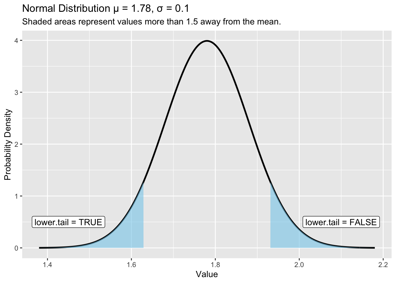
pnorm(lower.tail = TRUE), while the right tail corresponds to pnorm(lower.tail = FALSE).
Motivating scenario: You want to use R to calculate th probability that a draw from a normal falls in a certain range.
Learning goals: By the end of this chapter you should be able to:
pnorm() function to find the area in the upper or lower tail of any normal distribution, and understand its arguments.pnorm() to find the probability that a draw from a nromal lands in some predetermined area.
pnorm() to calculate a two-tailed p-value from a Z-statistic.pnorm()I introduced a webapp that integrates the area under the standard normal curve for you, and have shown that you can use rnorm() to simulate a normal distribution. Here, I introduce how to use pnorm() to have R, rather than my webapp, calculate this area.
This is useful because we often want to calculate a p-value, which amounts to asking “How much of the null sampling distribution is more extreme than my observed observed test statistic?”
pnorm()
pnorm(lower.tail = TRUE), while the right tail corresponds to pnorm(lower.tail = FALSE).
We can find the probability that a sample from a normal is greater than or less than some value of interest with R’s pnorm() function, which takes the arguments:
q: The value of interest.mean: The population mean, \(\mu\).sd: The population standard deviation, \(\sigma\).lower.tail: Whether we want the upper or lower tail (see Figure 1).
lower.tail = TRUE for the lower tail.lower.tail = FALSE for the upper tail.Now, try it yourself. Use the webR console below to calculate the probability that a random draw from our distribution (\(X \sim \mathcal{N}(1.78,\,0.01)\)) is
Remember the notation: \(\mathcal{N}(1.78,\,0.01)\) means a normally distributed random variable with mean 1.78 and variance 0.01 (i.e. standard deviation pod \(\sqrt{0.01}=0.1\)).
.
Less than 1.63: type pnorm(q = 1.63, mean = 1.78, sd = 0.1, lower.tail = TRUE) = 0.0668072.
Greater than 1.93: type pnorm(q = 1.93, mean = 1.78, sd = 0.1, lower.tail = FALSE) = 0.0668072.
If you got these answers right, you should have noticed that they are the same. This makes sense because the normal distribution is symmetric and both values are 1.5 standard deviations away from the mean.
The pnorm() function is a great tool, but it has one limitation: it only calculates the probability from a single point out to one of the tails. This is useful, but it doesn’t directly answer other common questions, like:
Fortunately, by combining results from pnorm() with two simple rules from probability theory we can answer these sorts of questions. Below we’ll cover:
Above we found that \(6.68\%\) of the normal distribution is 1.5 standard deviations less than the population mean. We also found that \(6.68\%\) of the normal distribution is 1.5 standard deviations greater than the population mean.
Because a single value cannot be in both the upper tail and the lower tail at the same time, these events are mutually exclusive. To find the total probability of either one OR the other happening, we simply add their individual probabilities.
\[P(A \text{ or }B) = P(A) +P(B)\] So the percent of samples from a normal are either 1.5 standard deviations more than or 1.5 standard deviations less than the mean equals \(0.0668 + 0.0668 = 0.1336\). Because these are symmetric we could have just multiplied \(0.0668\) by two. However this addition rule applies for any combination of mutually exclusive options.
The simple addition rule only applies to mutually exclusive events. For nonexclusive events we need to subtract off cases where both events happen to avoid double counting.
We just found that the probability of a value being more than one and a half standard deviations away from the mean is 0.1336. If we know the probability of an extreme outcome, what’s the probability of a “typical” outcome (i.e., not an extreme one)?
We can use the complement rule to answer this! Since the total probability of all possible outcomes must sum to 1, the probability of being within one and a half standard deviations is simply 1 minus the probability of being outside it.
For example, to find the probability of a value falling within 1.5 standard deviations of the mean for a standard normal distribution, we would calculate:
\[P(-1.5 < X < 1.5) = 1 - P(X < -1.5 \text{ or } X > 1.5) = 1 - 0.1336 = 0.8664\]
We will introduce many specific statistical tests in the following chapters. However, many of them can be approximated by a simple Z-test. The Z-test evaluates the null hypothesis (\(H_0\)) that a normally distributed test statistic is equal to a specific value.
To conduct a Z-test we:
2 * pnorm(q = abs(Z), lower.tail = FALSE).Finding the Z statistic should remind you of the Z-transform, but rather than transforming each data point, we transform our data summary. As such we subtract the proposed value under then null, \(\mu_0\), from our observed value, \(\bar{x}\), and divide buy the standard error (i.e. the standard deviation of the sampling distribution)
\[Z=\frac{\bar{x}-\mu_0}{\sigma_\bar{x}}\]