• 16. The “Paired” t-test

Motivating Example: You want to look into the differences between treatments in a great experiment in which pairs of otherwise identical individuals had a different treatment.

Learning Goals: By the end of this section, you will be able to:

• Identify the difference between “paired” and “unpaired” data.
• Explain the paired t-test as a one-sample t-test performed on the differences between pairs.
• Visualize paired data to highlight within-pair differences.
• Calculate and interpret a paired t-test in R, including the mean difference, confidence intervals, t-statistic, and p-value.
• Assess the assumptions of a paired t-test, focusing on the distribution of the differences.

Paired t-test

A common use of the one-sample t-test is to compare groups when there are natural pairs in each group. These pairs should be similar in every way, except for the difference we are investigating.

We cannot just pair random individuals and call it a paired t-test.

For example, suppose we wanted to test the idea that more money leads to more problems. We give some people $100,000 and others $1 and then measure their problems using a quantitative, normally distributed scale.

• If we randomly gave twenty people $100,000 and twenty people $1, we could not just randomly form 20 pairs and conduct a paired t-test.
  
• However, we could pair people by background (e.g., find a pair of waiters at similar restaurants, give one $100k and the other $1, then do the same for a pair of professors, a pair of hairdressers, a pair of doctors, and a pair of programmers, etc., until we had twenty such pairs). In that case, we could conduct a paired t-test.

Paired t-test Example:

I miss our parviflora plants too much - let’s get back to them. Recall that Brooke created “lines” (RILs) of parviflora plants. Although each RIL differed from all the others, each RIL can be replicated (by self fertilization), so Brooke planted genetically identical genotypes at each location.

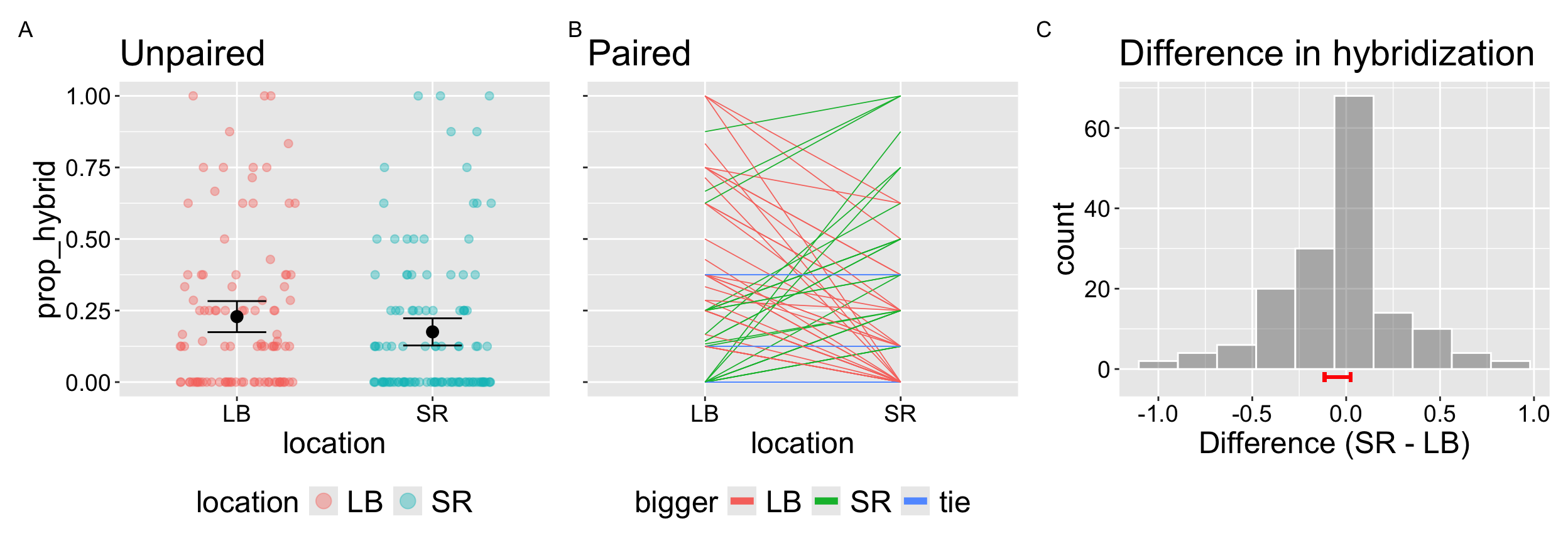
We can therefore test if the hybridization rate differed across locations. Here we focus on two locations – Lower Breckenridge (LB), and Sawmill Road (SR). The data are presented in Figure 1. Panels A and B show the same data in unpaired and paired form; panel C shows the distribution of within-RIL difference.

Below I introduce the paired t-test, which tests the null hypothesis that the mean difference between pairs is zero. To do so, we simply run a one sample t-test on the difference in values for each pair and test against the null of zero. This means our degrees of freedom equals the number of pairs minus one. Because this “pairing” accounts for differences across pairs and the paired t-test provides high statistical power to reject a false null hypothesis by focusing exclusively on differences within pairs.

The next chapter introduces the two-sample t-test. Although the two-sample t-test is less powerful than the paired t-test it is useful because it can be applied when data are not paired.

Figure 1: (A) Unpaired view: Hybridization proportion for each RIL at Lower Breckenridge (LB) and Sawmill Road (SR), with means ± 95% confidence intervals shown. (B) Paired view: Each line connects the same RIL grown at both sites. (C) The distribution of differences in hybridization rate for each RIL between sites (SR – LB). The red horizontal error bar shows the 95% confidence interval of the mean difference.

Evaluating assumptions

Because a paired t-test is simply a one-sample t-test on the differences in each pair, all our assumptions apply to the distribution of difference within pairs.

We know that data are independent, and collected without bias (way to go Brooke!). I also think that the mean seems like a reasonable summary of the data.

However, I know that the differences in each pair are not perfectly normal because:

• The original data are bounded between zero and one - so differences are bounded between negative one and one.
  
• The data are discrete – it’s one proportion minus another (each usually in increments of one eighth, as we usually assayed eight offspring).
  
• It also looks like there are an excess of zeros (i.e. the data are “zero inflated”) because many RILs made zero hybrids at both sites.

But we’re not looking for a perfect normal distribution. We want data to be normal enough so that we believe in our statistics. Because the t-test is robust to minor violations of assumptions of normality, and because our qq-plot (Figure 2) doesn’t look so bad, we can move on and do some stats.

ggplot(wide_lb_sr, aes(sample = diffs))+
  geom_qq(size = 4)+
  geom_qq_line()+
  theme(axis.text = element_text(size = 24),title  = element_text(size = 24),
        axis.title = element_text(size = 24),subtitle  = element_text(size = 18))+
  labs(title = "QQ-plot", subtitle = "Difference in hybridization",
       x = "Theoretical quantile", y= "Observed (SR - LB)")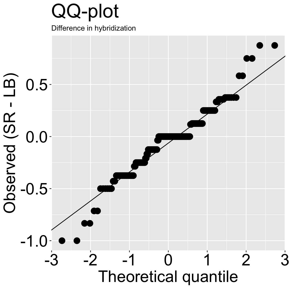

Figure 2: QQ-plot of differences in hybridization (Sawmill Road – Lower Breckenridge).

Summarizing data

While you are free to report means and confidence intervals for each “treatment” in a paired t-test, we are actually focused on the difference in pairs. In the tibble below, I have calculated this as:

\[\text{diffs} = \text{Prop hybrid}_\text{ Sawmill Road} - \text{Prop hybrid}_\text{ Lower Breckenridge}\]

So, we can now calculate the relevant summary stats:

diffs_summaries <- wide_LB_SR  |>
  summarise(n = n(),
            mean_diff = mean(diffs), 
            sd_diffs  = sd(diffs),
            cohens_D  = (mean_diff - 0) / sd_diffs,
            
            se_diffs  = sd_diffs / sqrt(n),
            t         = (mean_diff - 0) /  se_diffs)

n	mean_diff	sd_diffs	cohens_D	se_diffs	t
80	-0.046	0.312	-0.147	0.035	-1.317

🛑STOP🛑 Before we conduct a null hypothesis significance test you should immediately notice two things:

1. Any effect, if real is not particularly strong - a Cohen’s D value is “tiny” (0.01 – 0.20).
   
2. This will not be significant at the \(\alpha = 0.05\) level – results will never be statistically significant when t is less than 1.96.

But let’s move on to a formal test because we’re doing it.

The paired t-test in R

If your data are formatted like mine (see margin), the t.test function provides two equivalent ways to conduct a paired t-test. Both approaches give the same result, since they are just two ways of formulating the same test. I show you how to do them below:

• The one sample version: t.test(x = DIFFERENCES, mu = 0).
  
• The paired version: t.test(x = CONDITION ONE, y = CONDITION TWO, paired = TRUE).
  • For this version the \(i^{th}\) entry of x and y should refer to the same pair (pair, i).

Data for paired t-test

ril	LB	SR	diffs
A1	0.125	0.000	-0.125
A100	0.375	0.250	-0.125
A106	0.000	0.000	0.000
A111	0.000	0.125	0.125

One sample t-test version

t.test(x = pull(wide_LB_SR, diffs))

    One Sample t-test

data:  pull(wide_LB_SR, diffs)
t = -1.3171, df = 79, p-value = 0.1916
alternative hypothesis: true mean is not equal to 0
95 percent confidence interval:
 -0.11535736  0.02348236
sample estimates:
 mean of x 
-0.0459375 

Paired t-test version

t.test(x      = pull(wide_LB_SR, SR), 
       y      = pull(wide_LB_SR, LB), 
       paired = TRUE)

    Paired t-test

data:  pull(wide_LB_SR, SR) and pull(wide_LB_SR, LB)
t = -1.3171, df = 79, p-value = 0.1916
alternative hypothesis: true mean difference is not equal to 0
95 percent confidence interval:
 -0.11535736  0.02348236
sample estimates:
mean difference 
     -0.0459375 

Because our p-value exceeds 0.05 we fail to reject the null.

Concept check: We failed to reject the null. This means

The null is true The null is false The null is more likely to be true than false There is a p = 0.19 chance that the null is false There is a p = 0.19 chance that our results are due to sampling error Our sample did not provide strong evidence against the null hypothesis.