Motivating Scenario:
You are designing your study or critically evaluating someone else’s research. You know that a sample should be a random draw from a population, and that sampling bias can be a problem, but random sampling is a pain, and you are itching for more efficient ways to sample. You think you can (or the authors did) avoid sampling bias. What else should you worry about?
Learning Goals: By the end of this subsection, you should be able to:
Define statistical independence and non-independence.
Explain why non-independence is a problem.
Identify common sources of non-independence in biological data, such as genetic relatedness, spatial clustering, and experimental design flaws (e.g.pseudoreplication).
Non-independence and a False Sense of Confidence
We have seen that statistics has tools to deal with sampling error - random differences between the sample and the population, for example by quantifying uncertainty as the standard error. However, these tools assume that samples are independent.
A sample is independent - i.e. if knowing something about one observation gives you zero information about any other.
A sample is non-independent if observations are related or clustered.
Most of the statistics we do in this course relies on the assumption of independence. When we violate it, we can become wildly overconfident in our results, because our sample size isn’t what we think it is.
Below we walk through common sources of Non-Independence, anchoring most of this in the Clarkia System.
Later in the term, we will learn two approaches to mitigate non-independence: adding covariates to models and how to build mixed effect models. However, such statistical solutions increase uncertainty and can add additional complications, so it’s best to collect independent samples whenever possible.
Non-independence of measurements
I’m not sure if I said this already, but phenotypes from our Clarkia hybrid zones are actually not those of the plants we collected. Rather these data come from seeds collected from these plants.
The issue: At site GC we measured up to three offspring of each maternal plant. So we ended up with 239 data points from 87 moms. Because siblings resemble one another these data are non-independent.
We aimed to measure three kids per mom, but in some cases only one or two survived.
The consequence: If we naively used all 239 observations to generate a sampling distribution we would be overconfident in our estimates.
Potential solutions: So far, I’ve made these data independent by randomly choosing one kid per mom. An alternative approach would be to take the mean phenotype of the offspring, or two build a fancier model. For now I go with the random subsample because it is the most straightforward approach.
Pseudoreplication in Experimental Design
Let’s switch from our hybrid zone study to our RIL experiment. Recall that some RILs were pink-flowered and some were white-flowered. We planted the RILs at four field sites, and watched pollinator visitation and genotyped seeds to estimate the proportion of seeds on a flower that were hybrids.
Crucially we planted all RILs at all sites, but assume we didn’t. What would have happened if we planted pink-flowered plants at one site and white flowered plants at another?
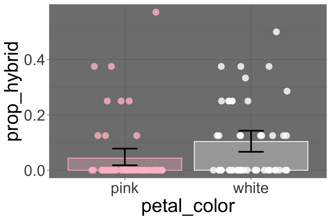
Let’s imagine that we planted pink flowered-plants only at “US” and white-flowered plants only at “LB”. As Figure 1 shows, in that case we would incorrectly and confidently conclude that white-flowered plants are more likely to set hybrid seed than are pink-flowered plants. This is why it is best to put spread treatments evenly across some background enviroenmnet when possible.
Figure 1: The proportion of hybrid offspring produced by pink- and white-flowered Clarkia plants. Because the pink-flowered and white-flowered plants were evaluated at different locations (“US” and “LG”, respectively), data are non-independent. This also creates a confounding bias.Error bars reflect 95% confidence intervals (see next chapter).
Psedudoreplication or sampling bias? It’s not clear to me if the example above is a case of pseudoreplication or sampling bias, it’s probably both.
This is clearly pseudoreplication because unearned confidence in our estimated hybrid seed proportion comes from the fact that our repeated measurements come from one location for each flower color. Thus our estimate of hybrid seed proportion is shielded from the variation across locations.
This is also a case of bias because the locations had different things going on which systematically altered the probability of hybrid seed set.
Returning to our survey of the natural hybrid zone at “GC” say that rather than conveniently sampling near the main road (as we did in the sampling bias section) you decide to do something that you hope will generate a random sample. You decide to use your computer to randomly select a location in the field site. You center a 1x1 meter quadrat and then sample every single plant inside it. You do this repeatedly (making minor adjustments in the case that the quadrat overlaps a previously sampled region to avoid double counting). Unfortunately, you are still sampling non-independently.
The Issue: This is a form of cluster sampling. As above, the plants within that one quadrat are not independent. They share the same microhabitat and are more likely to be the same subspecies or hybrid status than to plants 100 meters away.
The consequence: We would be more certain in our conclusions than we deserve.
Potential solutions: Just sample the plant in the grid closest to the randomly chosen point.
Non-independence generates a false sense of certainty. The core problem is that with non-independence your effective sample size — the number of independent pieces of information you have — is much smaller than the number of plants you measured.