• 16. t Summary

Links to: Summary. Chatbot tutor. Questions. Glossary. R packages. R functions. More resources.

Figure 1: T distribution adapted from xkcd. The rollover text sais “If data fails the teachers t-test you can force it to take it again until it passes.” See the related explainxkcd for more info!

Chapter summary

The t-distribution is a symmetric, bell-shaped curve defined by its degrees of freedom. Like the standard normal deviate, Z, the t-value measures the distance (in units of standard errors) between a sample estimate and a hypothesized population parameter. Compared to the Z-distribution, the t-distribution has “fatter tails,” reflecting the extra uncertainty from estimating the standard deviation.

We use the t-distribution to quantify uncertainty and to conduct a one-sample t-test of the null hypothesis that an approximately normally distributed sample came from a population with mean \(\mu_0\). A particularly useful application is the paired t-test. Here, each natural pair is split across two conditions, and we calculate differences in the response variable within each pair. The test then evaluates whether these differences are consistent with a null mean difference of \(\mu_0=0\).

Chatbot tutor

Please interact with this custom chatbot (link here). I have made to help you with this chapter. I suggest interacting with at least ten back-and-forths to ramp up and then stopping when you feel like you got what you needed from it.

Practice Questions

Try these questions! By using the R environment you can work without leaving this “book”. I even pre-loaded all the packages you need!

Part 1: Concepts

Q1. The difference between a t-value and a z-value is:

The z assumes the mean is zero, the t does not The z assumes that samples come from a normal distribution, the t does not The z assumes that we know the true population standard deviation, the t assumes we only have an estimate

---

Q2. If our sample is not perfectly normal:

We cannot use t-based tests, as the assume normality, and are not useful if data aren't normal We can use t-based tests so long as the sample is sufficiently large, and the deviations from normality aren't too big, so the central limit theorem bails us out. This has no impact on t - that's why we us a t-distribution instead of a z distribution

---

Q3. The t and z distributions will never be the exact same. But when will they be nearly identical?

When the sample size is large When the standard deviation is small When data are normal Never, these are very different distributions - this is akin to asking when an orange and apple are similar.

---

Q4. Which is the best summary of the effect size for normally distributed data?

The p-value The difference between the parameter and its null value The difference between the parameter and its null value, standardized by the standard deviation The difference between the parameter and its null value, standardized by the standard error

---

Part 2: Example

Figure 2: Paired differences in hyena “giggles” by dominance status. Each pair comprises one dominant and one subordinate hyena. Left: raw paired measurements with lines connecting each pair. Right: the within-pair difference (subordinate − dominant); points above 0 indicate more giggling by subordinates. The black point shows the mean difference with a 95% CI. Most pairs show positive differences, consistent with subordinates giggling more on average. (Data redrawn from Mathevon et al. 2010.)

Enjoy this video of hyena laughter.

---

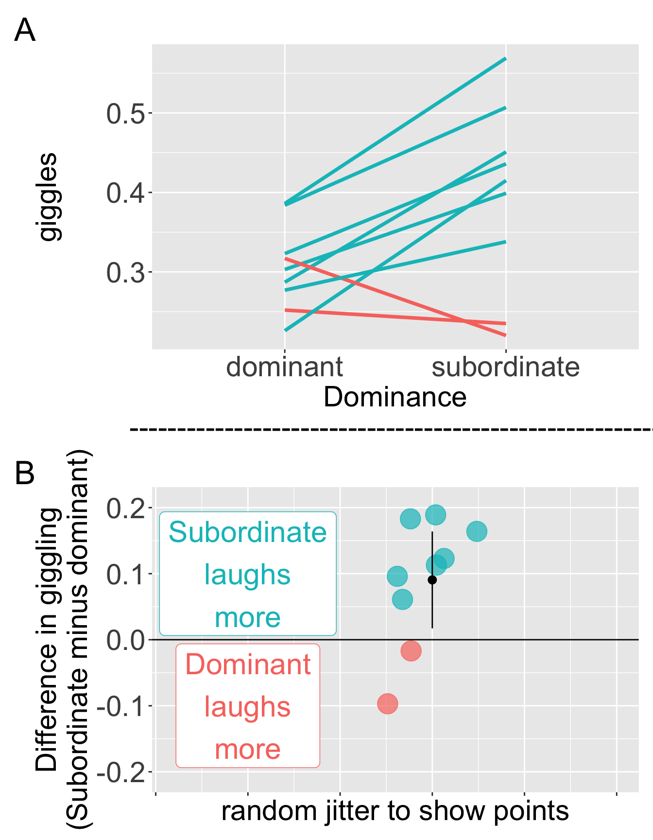
Setup. We’re not sure about the function of laughter, but there are some ideas that it could function to show dominance or subordinates. Mathevon and colleagues looked into this idea in hyenas. They found natural pairs of hyenas hanging out and noted which of the two was dominant and which was subordinate. They provided a measure of giggling (big number means more giggles). Because these data come naturally paired, we can conduct a t-test on the difference between pairs by testing the null hypothesis that this difference is zero. The data are available here, plotted in Figure 2, loaded below, and presented in Table 1:

Table 1

pair	dominant	subordinate	diffs
1	0.384	0.507	0.123
2	0.386	0.569	0.183
3	0.252	0.235	-0.017
4	0.226	0.415	0.189
5	0.323	0.436	0.113
6	0.287	0.451	0.164
7	0.303	0.399	0.096
8	0.317	0.220	-0.097
9	0.277	0.338	0.061

library(stringr);  library(dplyr); library(readr); library(ggplot2)
link <- "https://raw.githubusercontent.com/ybrandvain/datasets/refs/heads/master/chap12q23HyenaGiggles.csv"
hyenas<-read_csv(link) |>
 rename_all( str_remove, "IndividualGiggleVariation") |>
 mutate(diffs = subordinate - dominant)

Q5. Make a qq-plot. Then evaluate it in relation to the normality assumption.

The data are perfectly normal The data likely deviate somewhat from normality, but a t-test is probably ok The data deviate strongly from normality and any test assuming normality cannot be trusted

ggplot(hyenas, aes(sample = diffs))+
  geom_qq() +
  geom_qq_line()

---

For the next few questions, fill in the blanks to find:
- The standard deviation of the differences (sd_diff).
- Cohen’s d (cohens_d).
- The standard error (se_diff).
- The t-value (t).

Q6. The difference between in laughter between subordinate and dominant hyenas is ___ standard errors away from the zero. .

This is the t-value!

---

**Q7. The 95% CI is calculated as the mean ± ___ times the critical t-value at 𝛼= 0.05. Cohen’s dThe standard deviationThe variancetThe standard error1.96

---

Q8. To find this two tailed, 95% confidence interval, you must find the critical t-value. For this case the critical t-value equals (return the absolute value) .

We use the qt()function to find the critical t-value. There are two key arguments

• p: which equals \(\alpha/2\). Because we’re looking for the 95% confidence interval, \(\alpha = 1.00 -0.95 = 0.05\). So p = \(\alpha/2 =0.025\).

• df: The degrees of freedom, which equals \(n - 1\). Because \(n=9\), we have eight degrees of freedom.

qt() also takes an optional argument, lower.tail. Setting this to FALSE returns a poistive number.

---

Q9. Given the answers to Q7 and Q8 do you think the difference between subordinates and dominants is statistically significant at the \(\alpha = 0.05\) level?

yes because t is greater than the critical value no because t is greater than the critical value we can't know this until we find our p-value

---

Q10. Therefore, according to traditional statistical practice, we

Proceed as if the null is false (interpret results accordingly), while recognizing that there is a real chance we're wrong Proceed as if the null is true (interpret results accordingly), while recognizing that there is a real chance we're wrong Reserve all judgement until we prove that the null is true (or false)

---

Q11. Say you found a p-value of p. Which would be a correct interpretation of p?

p is the probability that the null hypothesis generated the data (or something more extreme). p is the probability that the null hypothesis is true. p is the probability that a random sample from the null hypothesis would be as or more extreme than the data

---

Q12. Say I had data from another two dominant individuals and another two subordinate individuals, but they were not from a pair. Would it be legit to randomly pair them and do a paired t-test? YesNo

📊 Glossary of Terms

• t-distribution: A continuous probability distribution, similar to the normal distribution but with heavier tails to account for uncertainty when the population standard deviation is unknown. Defined by its degrees of freedom.
• Degrees of Freedom (df): The number of independent values in a calculation that are free to vary. For a one-sample t-test, \(df = n-1\).
• Critical Value (\(t\_{\alpha/2, df}\)): The cutoff from the t-distribution that marks the boundary for rejecting the null hypothesis at a chosen significance level \(\alpha\).
• Effect Size: A quantitative measure of the magnitude of a phenomenon; here it describes how far the sample mean is from the null hypothesis mean, in standardized units.
  • Cohen’s d: A standardized effect size calculated as the mean difference divided by the sample standard deviation, \(d = (\bar{x} - \mu\_0)/s\).
• t-value: The distance in estimated standard errors between a sample estimate of the mean \(\bar{x}\), and its hypothesized value under the null hypothesis, \(\mu_0\).
  • t is calculated as \(\frac{\bar{x} - \mu_0}{s_\bar{x}}\), where \(s_\bar{x}\) is the estimate of the standard error (below).
  • t is the test statistic for a t-test.
    
• Standard Error (SE): An estimate of the standard deviation of the sampling distribution, calculated as \(s_\bar{x}=\frac{s}{\sqrt{n}}\) for the mean of a normal or t-distribution.
  
• One-Sample t-test: A test used to compare the mean of a single sample to a hypothesized population mean.
  
• Paired t-test: A test comparing the means of two related samples (e.g., before vs. after, or paired individuals), by analyzing the distribution of their differences.

---

🛠️ Key R Functions

• pt(): Finds cumulative probabilities for a t-distribution (area under the curve up to a value).

• qt(): Finds critical values (quantiles) for a t-distribution, e.g. for confidence intervals.

• t.test(): Performs one-sample, two-sample, or paired t-tests in R.

  • One sample” t.test(x = your_vector, mu = mu0).
    • You may need to pull() your vector from a column in a tibble.
      
    • \(\mu_0\) is the value of \(\mu\) under the null hypotheses
  • Paired: t.test(x = your_vector_of_diffs, mu = 0). OR t.test(x = vector_treat_a,y = vector_treat_b, paired = TRUE).

• lm(): Fits linear models; an intercept-only model (lm(y ~ 1)) is equivalent to a one-sample t-test.

geom_qq() and geom_qq_line(): Create QQ plots to visually check whether data are close enough to normal. - Remember to set aes(sample = THING) instead of aes(x = THING).

Additional resources

Videos:

• The Normal Distribution: Crash Course Statistics #19: A clear description of the normal disitrbution, how it arises, its properties, and the central lmit theorem. This is a nice summary of the key concepts in this chapter.

• But what is the Central Limit Theorem? from 3Blue1Brown’s youtube page]: An approachable introduction to more technical aspects of the normal distribution and the central limit theorm. This is the first video in his youtube playlist on the central limit theorem.

• Khan Academy Central Limit Theorem.