• 16. Assumptions of t
Motivating scenario: Statistical modelling allows us to test null hypotheses and quantify uncertainty. But results from these models are only as good as the data and the fit between data and assumptions of the analysis. Here we learn how to check these assumptions, and learn what to do when assumptions are violated.
Learning goals: By the end of this section, you should be able to:
- List and explain the assumptions made in using a t-distribution.
- Define what it means for a test to be “robust” to a violation of an assumption.
- Use your brain to think about the bias and independence of data.
- Use visual tools like a QQ plot lineup and a tile plot to see if data are normal enough to proceed.
- Make and justify a decision about if we are safe using a t-distribution after evaluating the assumptions of this distribution.
Assumptions in statistical models
Modeling uncertainty and testing null hypotheses requires an appropriate sampling distribution. But remember our challenge - we are stuck with a single sample so we don’t have a sampling distribution. To make this distribution, we must make some assumptions. For resampling methods like bootstrapping and permutation, we assume the data are independent and collected without bias. Parametric methods, like the t-test, use a well-defined statistical distribution (here, the t-distribution) as a shortcut to get a sampling distribution. This shortcut is only valid if its own assumptions are met. When using the t-distribution, we assume:
- Data are independent.
- Data are collected without bias.
- The mean is an appropriate summary of the data. AND
- Data are normally distributed.
What to Do When We Violate Assumptions
If our data meet assumptions, we can trust our inference. If data do not meet assumptions, the validity of our inferences is no longer guaranteed. Rather we must think hard about our data and what we know about our distribution to evaluate whether we can trust our inference (i.e. if our inferences are robust to violations of assumptions) or not.
The robustness of our inference depends on which assumptions are broken, and how severe any such violations are. For example, because the central limit theorem states any sampling distribution approaches the normal distribution as sample sizes get large the t-distribution is robust to modest deviations from normality. Here’s what to do if our data violate different assumption:
Bias is very difficult to address and is best managed by designing a better study. However, if you fully know the bias of the data, you can try an advanced technique to model this bias.
Whether the mean is a meaningful summary is a biological question, and a different summary could be evaluated by other methods. For example you could bootstrap the data and generate some other summary of the data if you want.
Non-independent data can be modeled, but such models are beyond the scope of this chapter.
The normality assumption is the easiest to address. If this assumption is violated, we can:
- Ignore it (if the violation is minor) because the central limit theorem helps us. OR
- Transform the data to an appropriate scale. OR
- Use bootstrapping to estimate uncertainty and/or conduct a binomial test, treating values greater than \(\mu_0\) as “successes” and less than \(\mu_0\) as “failures” (covered in future chapters).
- Ignore it (if the violation is minor) because the central limit theorem helps us. OR
Evaluating Assumptions for our Data
Are the data biased? Hopefully not, but this depends on the study design. For example, we might want to know if species had as much opportunity to increase in elevation as to decrease. How were the species selected? etc etc…
Is the mean a meaningful summary of the data? My sense is yes, but take a look and judge for yourself.
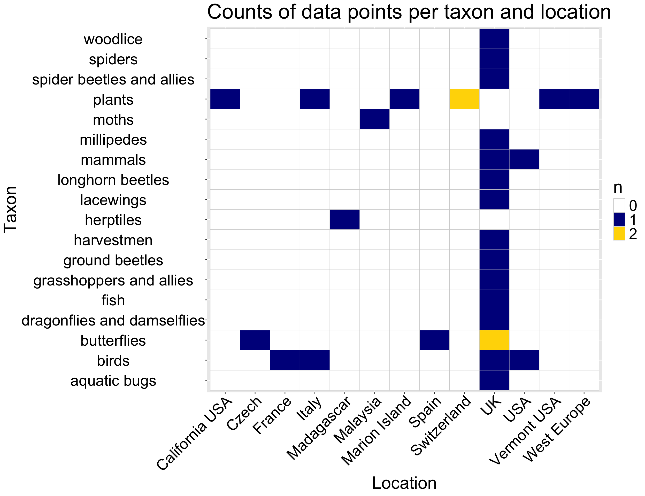
Are the data independent? I’m not sure about this. We see that some locations and some taxa are there more than once (Figure 1). My sense is this means the data are not actually independent. What if there’s something unique about low-elevation regions in the UK? This isn’t necessarily a reason to stop the analysis, but it’s worth considering.
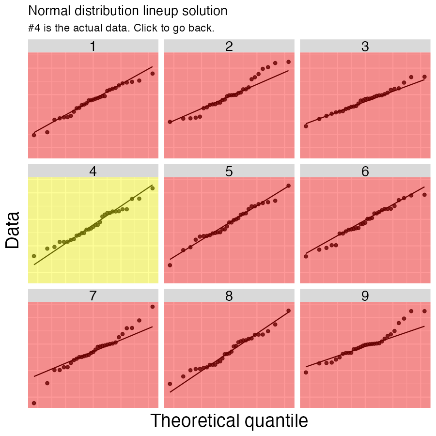
- Is the sample (or more specifically, the sampling distribution) normal? My sense is that the data are normal enough! But you can view the data and decide for yourself. As a guide, the image below displays nine quantile-quantile plots – one shows our data while the other eight were generated with
rnorm(). Can you easily tell which one is from the real data? I sure can’t, so this seems normal enough to me!
# Code for qq plot

range_shift|>
  ggplot(aes(sample = elevationalRangeShift))+
  geom_qq()+
  geom_qq_line()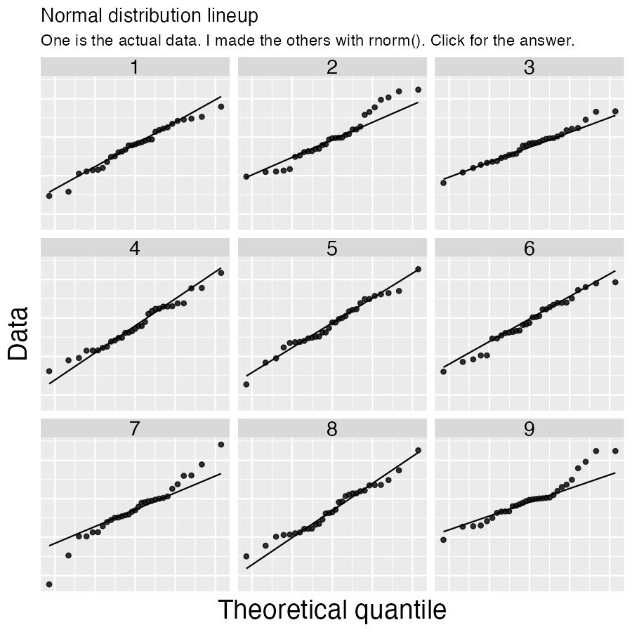
LFG
Although the data may not be fully independent, it roughly meets the assumptions of the t-distribution. Now that we’ve evaluated our assumptions let’s get to statin!