• 13. Statistical Significance
Motivating Scenario: You now can calculate a p-value and know what it means. But what do you do now? How do you present and report these results especially when you feel the need to make a clear decision about the trend.
Learning Goals: By the end of this section, you should be able to:
Understand the idea of statistical significance.
Explain why we never accept the null hypothesis.
Recognize that the result of null hypothesis significance testing is not the truth.
- We may reject a true null (At best we reject a true null with probability \(\alpha\), which by convention is set to 0.05).
- We may fail to reject a false null (we do so with probability \(\beta\)). Our “power” to reject false nulls is \(1-\beta\). The value of \(\beta\) depends on the effect size and sample size.
- We may reject a true null (At best we reject a true null with probability \(\alpha\), which by convention is set to 0.05).
Drawing a conclusion from a p-value.
So what do scientists do with a p-value? A p-value itself is an informative summary – it tells us the probability that a random draw from the null distribution would be as or more extreme than what we observed.
But here’s where things get weird. We use this probability as a measure of our data and the process that generated it.
- If our p-value is sufficiently small, we “reject” the null hypothesis and tentatively conclude that it did not generate our data.
This is a sneaky bit of logic that is not fully justified but seems to work anyways (see the next section).
- If our p-value is not sufficiently small, we “fail to reject” the null hypothesis, and tentatively conclude that there is not enough evidence to reject it.
What is “sufficiently small?” A glib answer is the greek letter, \(\alpha\). What should \(\alpha\) be? There is no real answer, and the value of \(\alpha\) is up to us as a scientific community. \(\alpha\) reflects a trade-off between the power to reject a false null and the fear of rejecting a true null. Despite this nuance, \(\alpha\) is traditionally set to 0.05, meaning that we have a 5% chance of rejecting a true null. This convention comes from a few words from RA Fisher such as this quote below from Fisher (1926) link here:
“. . . it is convenient to draw the line at about the level at which we can say: Either there is something in the treatment, or a coincidence has occurred such as does not occur more than once in twenty trials. . .”
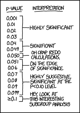
These customary rituals are taken quite seriously by some scientists. For certain audiences, the difference between a p-value of 0.051 and 0.049 is the difference between a non-significant and significant result—and potentially between publication or rejection. I, and many others (e.g., this article by Amrhein et al. (2019)), think this is a bad custom, and not all scientists adhere to it. Even Fisher himself seemed to waffle on this (link). Nonetheless, this is the world you will navigate, so you should be aware of these customs.
We never “accept” the null
By convention we never accept the null hypothesis – we simply “fail to reject” it. The reason for this is that we know that the null still may well be incorrect. In fact, the same effect size in a larger study would have more power to reject the null.
False positives and false negatives
|
p-value > α Fail to Reject H₀ |
p-value ≤ α Reject H₀ |
|
|---|---|---|
|
True null hypothesis (H₀ is TRUE) |
Fail to reject true null hypothesis Occurs with probability 1 - α This is the correct decision |
Reject true null hypothesis Occurs with probability α (Type I Error) |
|
False null hypothesis (H₀ is FALSE) |
Fail to reject false null hypothesis Occurs with probability β (Type II Error) |
Reject false null hypothesis Occurs with probability 1 - β (akaPower) This is the correct decision |
The table above should serve as a reminder that the result of the binary decision of a null hypothesis significance test does not cleanly map onto the truth of the null hypothesis.
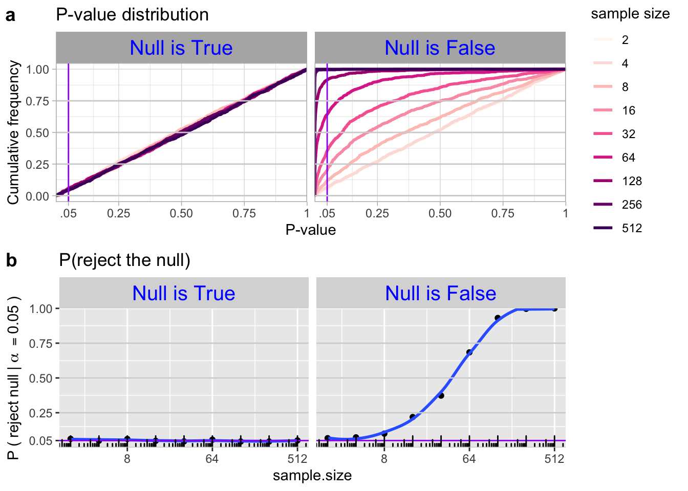
Rejecting the null does not mean that the null is untrue. The basic logic of null hypothesis significance testing means that we will reject a true null hypothesis 5% of the time (if \(\alpha\) is set to the conventional 0.05). This outcome is called a “false positive result”. When the null hypothesis is true, p-values will be uniformly distributed, and the false positive rate will be \(\alpha\) regardless of sample size (Figure 2).
Failure to reject the null does not mean that the null is true. We will occasionally fail to reject some false nulls. This occurs with probability \(\beta\). So, \(1-\beta\) is our so called “power” to reject a false null. Unlike our false positive rate, which always equals \(\alpha\), our false negative rate depends on both the sample size and the effect size. When the null hypothesis is false, we will observe more smaller p-values as the sample size increases, and the true positive rate will increase with the sample size (Figure 2).
We address this in some detail in the next subsection!