27. Probability and Likelihood
Motivating Scenario:
Learning Goals: By the end of this chapter, you should be able to:
A Very Brief Intro to Probability
A theme of this book (and of all of statistics) is that nothing is truly certain. Outcomes are not inevitable. Rather, each possible outcome in a “sample space” carries some probability.
This – of course – does not mean that all outcomes are equally probable. For example, in NHST we reject the null hypothesis when our observations (or something more extreme) are an improbable outcome of the null sampling distribution. As such, the rules of probability play a key role in NHST specifically and all of statistics, more broadly.
Probability: Terms and Conditions Apply
Conditional probabilities
There is a true probability that a specific outcome occurs. This “parameter” is the proportion of observations in an infinite number of trials that lead to our focal outcome. So \(P(A)\) is the probability that thing A occurs.
A simple example is a coin flip with two possible outcomes: heads or tails. If the coin is “fair” these outcomes are equally probable. So, we say:
\[P(\text{Heads} \mid \text{fair coin}) = 0.5\]
To unpack this notation a bit:

- \(P\) stands for probability.
- \(P(\text{Heads})\) shows which outcome we are considering (in this case, seeing heads),
- \(|\_\_\). The vertical bar “|” means “given” or “under the condition of.” This is the probability the coin shows heads, given that we know it is fair. Another word for this is that this is a conditional probability.
Of course, not all coins are fair. If I gave you a trick coin that came up heads 75% of the time, we would have:
\[P(\text{Heads} \mid \text{Yaniv's trick coin}) = \frac{3}{4}\].
As for any parameter, we almost never KNOW the true probability. Rather, we usually estimate it as the proportion \(\hat{p}\):
\[\widehat{p} = \frac{\# \text{ of times the focal outcome occurred}}{\# \text{ of trials}}\]
Independence and non-independence:
In some cases, knowing a condition does not provide additional information about the probability of the outcome. For example, my fair coin is equally likely to come up heads any day of the week. So:
\[P(\text{Heads} \mid \text{fair on monday}) = P(\text{Heads} \mid \text{fair on tuesday}) = 0.5\]
Here the probability of heads, \(P(\text{Heads})\), is independent of the day of the week. Other times, the condition matters. For example \(P\text{(rain | sunny)} \neq P\text{(rain | cloudy)}\). So, rain and clouds are not independent.
Combining probabilities
We are often interested in more complex probabilities. For example:
- What is the probability it rained or was cloudy?
- What is the probability it rained two days in a row?
Add probabilities to find the probability of “OR”
To find the probability that A OR B happened, we add the probability of A and the probability of B, and then subtract the probability of both happening so we don’t double-count:
\[P(\text{A OR B}) = P(\text{A}) + P(\text{B}) - P(\text{A AND B})\]
As a concrete example, consider the probability that it’s raining or cloudy. These aren’t mutually exclusive events—rain usually comes with clouds—so:
\[P(\text{rain OR cloudy})= P(\text{rain}) + P(\text{cloudy}) - P(\text{rain AND cloudy})\]
Here the term, \(P(\text{rain AND cloudy})\), is non-zero because it can be cloudy and rainy at the same time.
When A and B cannot happen at the same time (i.e., when they’re mutually exclusive), the overlap is zero. In that special case, the formula simplifies to:
\[P(\text{A OR B}) = P(\text{A}) + P(\text{B})\]
The last “OR” rule we need is the law of total probability. This says that the probability of some outcome is the sum of all the mutually exclusive ways that the outcome can occur. For example:
More broadly, the law of total probability states: \[P(B) = \sum P(B|A_i) \times P(A_i)\]
\[P(\text{rain}) = P(\text{rain AND sunny}) + P(\text{rain AND cloudy})\] \[=P(\text{rain | sunny})\times P(\text{sunny}) + P(\text{rain | cloudy})\times P(\text{cloudy})\]
Seeing this idea to its logical conclusion, the probabilities of all mutually exclusive outcomes have to add up to one. For example if each day is either sunny or cloudy, but not both or neither, \(P(\text{sunny}) + P(\text{cloudy}) = 1\).
This leads to the rule for NOT: the probability of not having some outcome is simply one minus the probability of that outcome:
Here we treat “sunny” and “cloudy” as mutually exclusive conditions. Of course, real weather can include things like “partly sunny,” “partly cloudy,” or days with both sun and clouds etc… We’re ignoring those complications for now to keep the example simple.
\[P(\text{NOT A}) = 1 - P(A)\]
Multiply probabilities for the probability of AND
To find the probability that two things happen together, we multiply the probability of one event (say A) by the probability of the second event given that the first one has already happened.
\[P(\text{A AND B}) = P(A)\times P(B|A) = P(B)\times P(A|B)\]
For example, the probability that it is raining and cloudy is \(P(\text{rain AND cloudy})= P(\text{cloudy})\times P(\text{rain | cloudy})= P(\text{rain})\times P(\text{cloudy | rain})\)
Bayes’ theorm: Flipping conditional probabilities
If we know it’s not raining, we can use “Bayes’ Theorem” to flip these conditional probabilities. For example, we can use Bayes’ theorem to find the probability it’s sunny given that it’s not raining. I find that the easiest way to think about it is as follows:
Find the expected number of rain-free sunny days in a year. This will be our numerator.
Find the number of rain-free days in a year. This will be our denominator
\[P(\text{Sunny | No rain}) = \frac{\#\text{ sunny rain-free days}}{\# \text{rain-free days}}= \frac{\cancel{365} \times P(\text{No rain AND sunny}) }{\cancel{365} \times P(\text{No rain})}\]
The 365 is there to get days in a year. This helps me think concretely - but is mathematically unnecessary (because it’s in the numerator and denominator) and cancels out.
Now we simply apply our rules from above:
Multiplication rule: \(P(\text{No rain AND sunny}) = P(\text{No rain | sunny }) \times P(\text{sunny})\).
Law of Total Probability: \(P(\text{No rain})\) \(=P(\text{No rain AND sunny}) + P(\text{No rain AND cloudy})\) \(=P(\text{No rain | sunny }) \times P(\text{sunny}) +P(\text{No rain | cloudy }) \times P(\text{cloudy})\).
\[P(\text{Sunny | No rain}) = \frac{P(\text{No rain | sunny }) \times P(\text{sunny})}{P(\text{No rain | sunny }) \times P(\text{sunny}) +P(\text{No rain | cloudy }) \times P(\text{cloudy})}\]
More broadly, Bayes’ theorem allows us to flip conditional probabilities as:
\[P(A|B) = \frac{P(B|A) \times P(A)}{P(B)}\]
Likelihood-Based Inference
The brief intro to probability theory, above, could have helped our statistical understanding up until now. But I think we did OK with the probability intuition and knowledge you already had. However, probability isn’t just for thinking about sampling distributions, we can use probability theory to develop richer and more flexible statistical analyses.
Specifically, we can use probabilities in “likelihood based inference” to go beyond the assumptions of linear models and build inferences under any model we can describe through an equation. This approach allows us to model more complex scenarios, like phylogenies, genome sequences, or any structured data. For now, however, we’ll stick to our simple normal distribution so that we can follow along.
Probabilities and Likelihoods
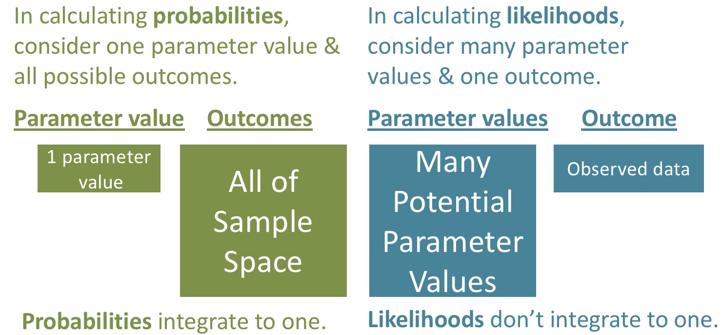
A probability represents the proportion of times a model would produce a particular result if we did the same thing many many times.
- When thinking about probabilities, we consider one model and all possible outcomes. For a given model, all probabilities (or probability densities) sum (or integrate) to one.
Mathematically, calculating a likelihood is identical to calculating a probability. The key difference lies in our perspective.
- With likelihood, we view the outcome as fixed and consider the various models that might have generated it.
In this way, a likelihood represents a conditional probability.
\[P(\text{Data} | \text{Model}) = \mathscr{L}(\text{Model} | \text{Data})\]
Log-Likelihoods
If our data points are independent, we can calculate the likelihood of all data points by taking the product of each individual likelihood. However, this approach introduces some practical challenges:
- Multiplying many probabilities often results in very small numbers, which can become so small that computers struggle to handle them accurately (underflow).
- Products of probabilities are also less convenient in mathematical operations – (remember the central limit theorem works when we add bits, not when we multiply bits).
To address these issues, we typically take the log of each likelihood and sum them all. In log space, addition replaces multiplication — for example, 0.5 * 0.2 = 0.1 becomes log(0.5) + log(0.2) = -2.302585, and \(e^{-2.302585} = 0.1\). So you will almost always see people talking about log-likelihoods instead of raw likelihoods.
Log Likelihood of \(\mu\)
How can we calculate likelihoods for a parameter of a normal distribution? Here’s how!
Suppose we have a sample with values 0.01, 0.07, and 2.2, and we know the population standard deviation is one, but we don’t know the population mean. We can find the likelihood of a proposed mean by multiplying the probability of each observation, given the proposed mean. For example, the likelihood of \(\mu = 0 | \sigma = 1, \text{ and } Data = \{0.01, 0.07, 2.2\}\) is:
dnorm(x = 0.01, mean = 0, sd = 1) *
  dnorm(x = 0.07, mean = 0, sd = 1) *
  dnorm(x = 2.20, mean = 0, sd = 1)
[1] 0.00563186A more compact way to write this is
dnorm(x = c(0.01, 0.07, 2.20), mean = 0, sd = 1) |>
  prod()
[1] 0.00563186Remember, we multiply because we assume that all observations are independent.
As discussed above, we typically work with log likelihoods rather than linear likelihoods. Because multiplying on the linear scale is equivalent to adding on the log scale, the log likelihood in this case is:
dnorm(x = c(0.01, 0.07, 2.20), mean = 0, sd = 1, log = TRUE) |>
  sum()
[1] -5.179316Reassuringly, \(ln(0.00563186) =\) -5.1793155, and similarly \(e^{5.179316} =\) 0.0056319
The Likelihood Profile
We can consider a range of plausible parameter values and calculate the (log) likelihood of the data for each of these “models.” This is called a likelihood profile. We can create a likelihood profile with the following:
obs            <- c(0.01, 0.07, 2.2)    # our observations
proposed.means <- seq(-1, 2, .001)      # proposing means from -1 to 2 in 0.001 increments

likelihood_profile <- tibble(proposed_mean = proposed.means)|>
  group_by(proposed_mean)|>
  # find the loglikelihood of each proposed "model"
  mutate(log_lik = sum(dnorm(x = obs, mean = proposed_mean , sd = 1, log = TRUE)))|>
  ungroup()
Now you can scroll through and see the log likelihoods of each proposed mean
Above I just said the standard deviation was one. But more often we find it from our data. However
The standard deviation in our likelihood calculations is a bit different than we are used to.
- First, we consider our sums of squares as deviations away from the proposed mean, rather than the estimated mean.
- Second we divide by n, not not n-1 (because we state the mean and do not estimate it)
Maximum Likelihood Estimate
How can we use this for inference? One estimate of our parameter is the value that “maximizes the likelihood” of our data (e.g., the x-value corresponding to the highest point on the plot above).
To find the maximum likelihood estimate, we find the biggest value (i.e. the smallest negative number) in our likelihood profile. We can find this by arranging our data set from largest to smallest number
likelihood_profile%>%
  arrange(desc(log_lik))
Or by filtering our data so we only have the proposed mean that maximizes the likelihood of our data
MLE <- likelihood_profile %>%
  filter(log_lik == max(log_lik))
# A tibble: 1 × 2
proposed_mean log_lik
<dbl> <dbl>
1 0.76 -4.31This equals the mean of our observations: mean(c(0.01, 0.07, 2.2)) = 0.76. In general, for normally distributed data, the maximum likelihood estimate of the population mean is the sample mean.
NOTE The maximum likelihood estimate is not the parameter with the best chance of being correct (that’s a Bayesian question); rather, it’s the parameter that, if true, would have the greatest likelihood of producing our observed data.
Likelihood based inference: Uncertainty and hypothesis testing.
Uncertainty
We need one more trick to use the likelihood profile to estimate uncertainty – log likelihoods are roughly \(\chi^2\) distributed with degrees of freedom equal to the number of parameters we’re trying to guess (here, just one – corresponding to the mean). So for 95% confidence intervals are everything within qchisq(p = .95, df =1) /2 = 1.92 log likelihood units of the maximum likelihood estimate.
in95CI <- pull(MLE, log_lik) -1.92

CI <- likelihood_profile             |>
  filter(log_lik > in95CI)           |>
reframe(CI = range(proposed_mean))| CI |
|---|
| -0.371 |
| 1.891 |
Now we can plot our likelihood profile, noting our MLE (in red) and 95% confidence intervals (the shaded area):
ggplot(likelihood_profile)+
  geom_rect(data = .  %>% summarise(ymin = min(log_lik),ymax = max(log_lik),
                                 xmin = min(pull(CI )),xmax = max(pull(CI ))),
            aes(xmin = xmin,xmax = xmax, ymin = ymin, ymax = ymax),
            fill= "lightgrey", alpha = .4)+
  geom_line(aes(x = proposed_mean, y = log_lik))+
  geom_vline(xintercept = pull(MLE, proposed_mean), color = "red")+
  theme_light()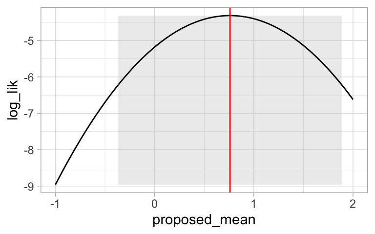
Null hypothesis significance testing.
We can find a p-value and test the null hypothesis by comparing the likelihood of our MLE (\(log\mathscr{L}(MLE|D)\)) to the likelihood of the null model (\(log\mathscr{L}(H_0|D)\)). We call this a likelihood ratio test, because we divide the likelihood of the MLE by the likelihood of the null – but we’re doing this in logs, so we subtract rather than divide. For this arbitrary example, lets pretend we want to test the null that the true mean is zero:
Log likelihood of the MLE: \(log\mathscr{L}(MLE|D)\) = Sum the log-likelihood of each observation under the MLE =
pull(MLE, log_lik)= -4.313.Log likelihood of the Null: \(log\mathscr{L}(H_0|D)\) = Sum the log-likelihood of each observation under the null =
likelihood_profile %>% filter(proposed_mean == 0)%>% pull(log_lik)= -5.179.
We then calculate \(D\) which is simply two times this difference in lof likelihoods, and calculate a p-value with it by noting that \(D\) is \(\chi^2\) distributed with degrees of freedom equal to the number of parameters we’re inferring (here, just one – corresponding to the mean). We see that our p value is greater than 0.05 so we fail to reject the null.
log_lik_MLE <- pull(MLE, log_lik)
log_lik_H0  <- likelihood_profile |>
  filter(proposed_mean == 0) |>
  pull(log_lik)
D      <- 2 * (log_lik_MLE - log_lik_H0)
p_val <- pchisq(q = D, df = 1, lower.tail = FALSE)| D | p_val |
|---|---|
| 1.733 | 0.188 |
Unfortunately, the LRT test give poorly calibrated p-values – especially when we have a small sample size.
Compare our LRT p-value of 0.188 to that’s from a one sample t-test
t.test(obs,mu=0)   |>
  tidy()           |>
  pull(p.value)
[1] 0.401964A simple solution is applying “Bartlett’s Correction for Small Samples” correction, here \(D_\text{corrected} = \frac{D}{1+\frac{1}{2\times n}}\). This gets us closer, but we still must recognize that the LRT is a very rough approximtation
This correction is necessary because, with small samples, the \(\chi^2\) approximation breaks down because the log-likelihood surface is not close to quadratic. With large samples, the LRT behaves extremely well.
Bartlett_D      <- D / (1+1/(2 * length(obs)))
Bartlett_p_val  <- pchisq(q = Bartlett_D, df = 1, lower.tail = FALSE)
print(Bartlett_p_val)
[1] 0.2229538Example 1: Are species moving uphill?
Chen et al. (2011) tested the idea that organisms move to higher elevation as the climate warms. To test this, they collected data (available here) from 31 species, plotted below (Figure 2).
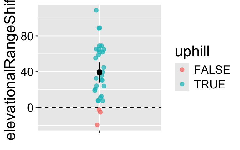
We could conduct a one sample t-test against of the null hypothesis that there has been zero net change on average.
lm(elevationalRangeShift ~ 1, data = range_shift) |>
tidy() |> mutate(p.value = p.value* 10^8)%>%mutate_at(2:5, round, digits = 2) %>% mutate(p.value = paste(p.value,"x 10^-8"))|> gt()| term | estimate | std.error | statistic | p.value |
|---|---|---|---|---|
| (Intercept) | 39.33 | 5.51 | 7.14 | 6.06 x 10^-8 |
Calculate log likelihoods for each model
There is nothing wrong with that one-sample t-test, but let’s use this as an opportunity to learn about how to apply likelihood. First we grab our observations, write down our proposed means – lets say from negative one hundred to two hundred in increments of .01.
observations   <-  pull(range_shift, elevationalRangeShift)
proposed_means <- seq(-100,200,.01)
n               <- length(observations)
We then go on to make a likelihood surface by.
Making a vector of proposed means
Calculate the population standard deviation (sigma) for each proposed parameter value,
For each proposed mean, find the log likelihood of each observation (with
dnorm)Sum the log likelihoods of each observation for a given proposed mean to find the log likelihood of that parameter estimate given the data.
Just for fun well arrange them with the MLE on top!
log_lik_uphill <- tibble(mu = proposed_means)%>%      # Step 1
  group_by(mu)%>%                                        # R stuff to make sure we only work within a parameter
  mutate(sigma   = sqrt(sum((observations-mu)^2) / n) ,  # Step 2: Find the standard deviation
         log_lik = dnorm(x = observations,               # Step 3: Find the
                         mean = mu,                      #    log-likelihood
                         sd = sigma,                     #    if each data
                         log= TRUE)%>%                   #    point
           sum())%>%                                     # Step 4: Sum the log-likelihoods
  ungroup()%>%
  arrange(desc(log_lik))
Log likelihoods of for 100 proposed means (a subst of those investigated above), sorted from highest to lowest log likelihood.
MLE
This sorted list shows that our maximum likelihood estimate is about 39 meters. The actual MLE is about
MLE <- log_lik_uphill %>%
filter(log_lik == max(log_lik))| mu | sigma | log_lik |
|---|---|---|
| 39.3 | 30.2 | -149.6 |
95% CI
Again, because log likelihoods are roughly \(\chi^2\) distributed with one degree of freedom, everything within qchisq(p = .95, df =1) /2 = 1.92 log likelihood units of the maximum likelihood estimate is in the 95% confidence interval:
in95CI <- pull(MLE, log_lik) -1.92

CI <- log_lik_uphill  %>%
  filter(log_lik > in95CI) %>%
reframe(CI = range(mu))| CI |
|---|
| 28.38 |
| 50.28 |
Now we can plot our likelihood profile, noting our MLE (in red) and 95% confidence intervals (the shaded area):
ggplot(log_lik_uphill)+
  geom_rect(data = .  %>% summarise(ymin = min(log_lik),ymax = max(log_lik),
                                 xmin = min(pull(CI )),xmax = max(pull(CI ))),
            aes(xmin = xmin,xmax = xmax, ymin = ymin, ymax = ymax),
            fill= "lightgrey", alpha = .4)+
  geom_line(aes(x = mu, y = log_lik))+
  geom_vline(xintercept = pull(MLE, mu), color = "red")+
  theme_light()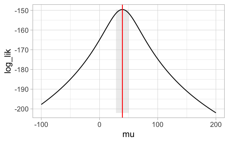
Null hypothesis significance testing.
As above we find the p-value by comparing two times the difference in log likelihoods under the MLE and the null model (\(D\)), to the \(\chi^2\) distribution with one degress of freedom. This value is in the same ballpart as what we got from the one sample t-test (\(6.06 \times 10^{-8}\))
log_lik_MLE <- pull(MLE, log_lik)
log_lik_H0  <- log_lik_uphill %>% filter(mu == 0)%>% pull(log_lik)
D      <- 2 * (log_lik_MLE - log_lik_H0)
p_val <- pchisq(q = D, df = 1, lower.tail = FALSE)| log_lik_MLE | log_lik_H0 | D | p_val |
|---|---|---|---|
| -149.59 | -164.99 | 30.79 | 2.87 x 10^-8 |
R tricks
You can grag the log likelihoods of a model with the logLikfunction.
MLE_model <- lm(elevationalRangeShift ~ 1, data = range_shift) # Estimate the intercept
logLik(MLE_model ) %>% as.numeric()
[1] -149.5937Null_model <- lm(elevationalRangeShift ~ 0, data = range_shift) # Set intercept to zero
logLik(Null_model ) %>% as.numeric()[1] -164.9888Or with the glance() function from broom
library(broom)
glance(MLE_model) %>% select(logLik) %>% pull()
[1] -149.5937You can also use the lrtest function in the lmtest package to conduct this test:
library(lmtest)
lrtest(Null_model,MLE_model )
Likelihood ratio test
Model 1: elevationalRangeShift ~ 0
Model 2: elevationalRangeShift ~ 1
#Df LogLik Df Chisq Pr(>Chisq)
1 1 -164.99
2 2 -149.59 1 30.79 0.00000002875 ***
---
Signif. codes: 0 '***' 0.001 '**' 0.01 '*' 0.05 '.' 0.1 ' ' 1Bayesian inference
We often care about how probable our model is given the data, rather than the reverse. Likelihoods can help us approach this! Remember Bayes’ theorem:
\[P(\text{Model|Data}) = \frac{P(\text{Data|Model}) \times P(\text{Model})}{P(\text{Data})}\]
Taking this apart:
- \(P(\text{Model|Data})\): The posterior probability—the probability of our model after observing the data.
- \(P(\text{Data|Model})\): The likelihood, which we’ve just calculated. Mathematically, it’s written as \(\mathscr{L}(Model|Data)\).
- \(P(\text{Model})\): The prior probability—our belief about the model’s probability before observing the data. Since we often don’t know this, we usually assign a value that seems reasonable.
- \(P(\text{Data})\): The evidence, or the probability of the data. This is calculated using the law of total probability.
Today, we’ll assign an arbitrary prior probability for demonstration purposes. This is not ideal—Bayesian inferences are only meaningful to the extent that we can meaningfully interpret the posterior, which depends on having a well-justified prior. However, for the sake of this example, let’s assume a prior: the parameter is normally distributed with a mean of 0 and a standard deviation of 30.
bayes_uphill <- log_lik_uphill |>
  mutate(lik   = exp(log_lik),
         prior = dnorm(x = mu, mean = 0, sd = 30) / sum(dnorm(x = mu, mean = 0, sd = 30) ),
         evidence  = sum(lik * prior),
posterior = (lik * prior) / evidence) 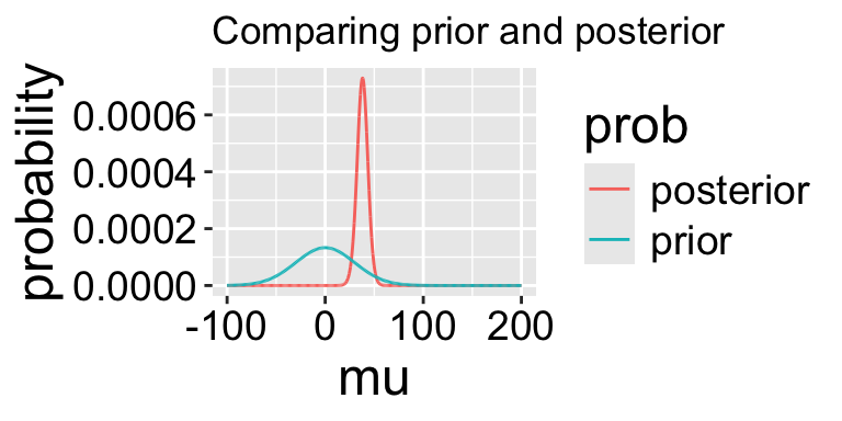
We can grab interesting thing from the posterior distribution.
- For example we can find the maximum a posteriori (MAP) estimate as
bayes_uphill |>
  filter(posterior == max(posterior))                                                                                                  |> data.frame()
mu sigma log_lik lik prior evidence posterior
1 38.08 30.19035 -149.6203 1.048907e-65 0.00005944371 8.550126e-67 0.0007292396Note that this MAP estimate does not equal our MLE as it is pulled away from it by our prior.
- We can grab the 95% credible interval. Unlike the 95% confidence intervals, the 95% credible interval has a 95% chance of containing the true parameter (if our prior is correct).
bayes_uphill                                  |>
  mutate(cumProb = cumsum(posterior))         |>
  filter(cumProb > 0.025 & cumProb < 0.975)   |>
  summarise(lower_95cred = min(mu),
            upper_95cred = max(mu))                                                                                                               |> data.frame()
lower_95cred upper_95cred
1 26.18 52.48Prior sensitivity
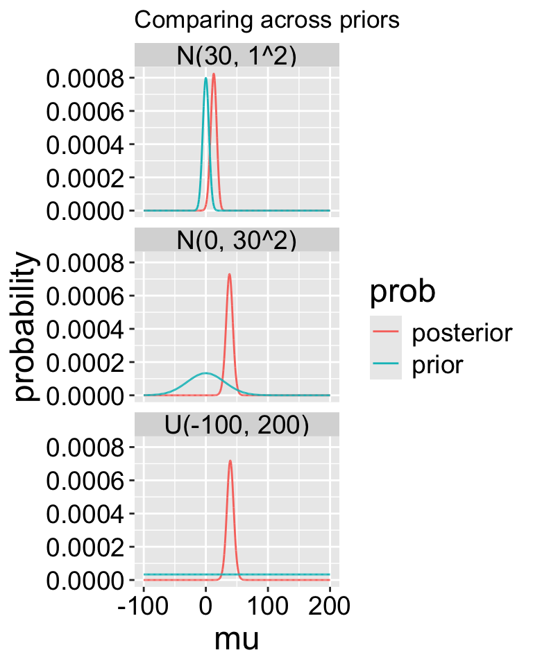
In a good world our priors are well calibrated.
In a better world, the evidence in the data is so strong, that our priors don’t matter.
A good thing to do is to compare our posterior distributions across different prior models. The plot below shows that if our prior is very tight, we have trouble moving the posterior away from it. Another way to say this, is that if your prior believe is strong, it would take loads of evidence to gr you to change it.
MCMC / STAN / brms
With more complex models, we usually can’t use the math above to solve Bayesian problems. Rather we use computer ticks – most notably the Markov Chain Monte Carlo MCMC to approximate the posterior distribution.
The programming here can be tedious so there are many programs – notable WINBUGS, JAGS and STAN – that make the computation easier. But even those can be a lot of work. Here I use the R package brms, which runs stan for us, to do an MCMC and do Bayesian stats. I suggest looking into this if you want to get stared, and learning STAN for more serious analyses
library(brms)
change.fit <- brm(elevationalRangeShift ~ 1,
    data   = range_shift,
    family = gaussian(),
    prior  = set_prior("normal(0, 30)",
                      class = "Intercept"),
    chains = 4,
    iter   = 5000)

change.fit$fit| term | mean | se_mean | sd | 2.5% | 25% | 50% | 75% | 97.5% | n_eff | Rhat |
|---|---|---|---|---|---|---|---|---|---|---|
| b_Intercept | 37.82 | 0.06 | 5.69 | 26.56 | 34.11 | 37.86 | 41.59 | 48.82 | 7863 | 1 |
| sigma | 31.70 | 0.05 | 4.25 | 24.84 | 28.68 | 31.24 | 34.20 | 41.34 | 6444 | 1 |
| lp__ | -156.70 | 0.02 | 1.04 | -159.48 | -157.09 | -156.38 | -155.97 | -155.70 | 4340 | 1 |