• 12. Uncertainty summary – Applied Biostatistics

Chapter summary

In the previous chapter, we saw that knowing the sampling distribution is the key to quantifying sampling error. However, we never have access to the true sampling distribution because that would require knowing the entire population—at which point we wouldn’t need to estimate uncertainty at all. Bootstrapping is a solves this problem by allowing us to approximate the sampling distribution using only our own sample. Bootstapping by repeatedly resampling our data with replacement to create thousands of new samples. The resulting bootstrap distribution of estimates can then be used to quantify uncertainty, for example by calculating the bootstrap standard error (the standard deviation of the bootstrap distribution) or by finding the X% confidence interval to provide a range of plausible values for the true population parameter.

A two-panel comic by @epilielle explaining the correct interpretation of confidence intervals. **Panel 1:** Says "People think confidence intervals are like archery," and shows a variable "true value" (an arrow) being shot at a fixed "confidence interval" (a target). **Panel 2** says: "But really confidence intervals are more like ring toss," and shows a variable "confidence interval" (a ring) being tossed at a fixed "true value" (a post), illustrating that the parameter is fixed while the interval is what varies and might capture it. — Figure 1: Understanding confidence intervals is tricky. This cartoon by Ellie Murray is the best explanation I have found to date. I copy and paste directly from her medium post “I’ve often heard students mis-use the target analogy to describe their confidence interval as if it were the fixed target, and the ”true” value was the arrow that may or may not land on the target 95% of the time…. But, a confidence interval isn’t fixed — the ”true” value is the part they should view as fixed. To avoid this misunderstanding, I like to explain confidence intervals with ring toss. The ”truth” is in a fixed place, and it’s the confidence interval ring that may or may not land where you want it to… A side benefit: this analogy can help students see why a 99% confidence interval would be wider than a 95% interval — the bigger the ring, the easier the game of ring toss!”. While we’re at it, Ishould mention that Ellie Murray co-host’s a fantastic podcast called “Casual inference”.

Chatbot tutor

Please interact with this custom chatbot (link here). I have made to help you with this chapter. I suggest interacting with at least ten back-and-forths to ramp up and then stopping when you feel like you got what you needed from it.

Practice Questions

Try these questions! By using the R environment you can work without leaving this “book”. I even pre-loaded all the packages you need!

Q1) The ___ is the key idea we use to think about uncertainty due to sampling error. .

The Sampling distribution is the foundation idea for thinking about uncertainty. It’s a the distribution sample estimates, and it’s what allows us to think about the nature of sampling error.

If you chose “Standard error”: You’re on the right track! The standard error is how we quantify or measure the uncertainty. However, the sampling distribution is the larger idea or conceptual framework that allows us to understand where that standard error comes from.

If you chose “Bootstrap distribution”: This was a tricky one! The bootstrap distribution is a fantastic tool we use to approximate the sampling distribution when we only have one sample. The sampling distribution is the true, underlying theoretical idea that we are trying to estimate with the bootstrap.

If you chose “Standard deviation”: This is a very common point of confusion, as the two terms are closely related! A standard deviation measures the spread or variability of individual data points within your single sample. The standard error measures the variability of a sample estimate (like the sample mean) across many different potential samples (which is what the sampling distribution shows). So, standard deviation describes your data’s variability, while the standard error describes the uncertainty of your estimate due to sampling.

Come on. What are you even thinking.

Q2) For real data, we can use the _, which we make by sampling replacement to estimate with uncertainty.

Q3) Which of these estimates tend to get bigger as sample sizes got smaller? (there is more than one right answer. find them all). HINT: playing with this webapp can help.

Our uncertainty decreases with increasing sample size.

If you chose “Standard deviation” or “Mean”: That’s a great thought, because estimates of the mean and standard deviation are definitely less precise with smaller samples! However, their values don’t systematically get bigger or smaller. A sample mean from a small sample is just as likely to be above the true population mean as it is below. Likewise, the standard deviation of your sample is your best guess for the spread of the whole population, and that guess doesn’t have a tendency to get bigger, just less reliable.

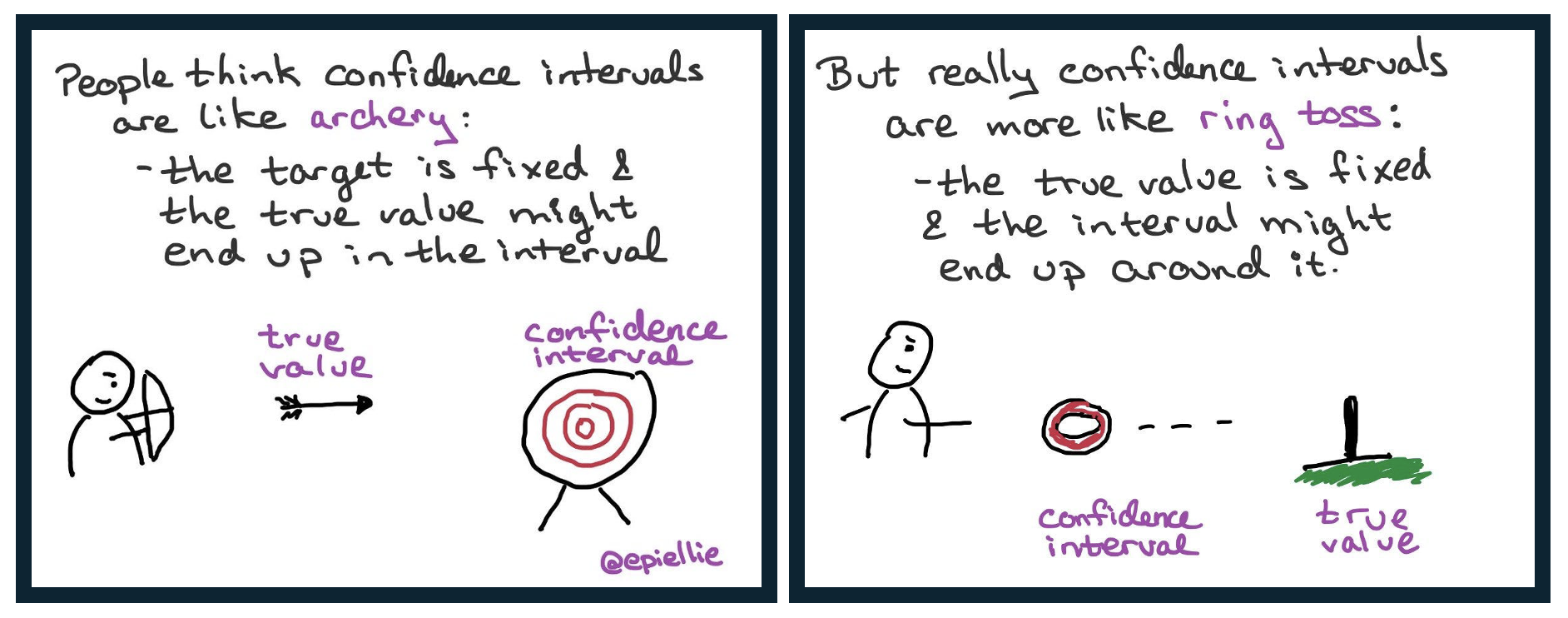
Q4) You calculated a 95% confidence interval from a random sample. What is the probability that the confidence interval captured the true population parameter? (check all that apply).

The true population parameter is also a single, fixed number. Once you have taken your sample and calculated the confidence interval, that interval is a fixed range of numbers (e.g., 0.108 to 0.199). At this point, your fixed interval either contains the fixed parameter or it does not. The “chance” part of the process is over.

The 95% refers to the long-run success rate of the method you used. It means that if you were to repeat your entire sampling process 100 times, you would expect about 95 of the resulting confidence intervals to capture the true parameter. It does not apply to any single, already-calculated interval.

The sample size and variability influence the width of the confidence interval, not its interpretation!

Q5) You actually know the population parameter. A bunch of friends sample randomly from this population, and calcualte 95% confidence intervals. What proportion of these confidence intervals will catch the true parameter? (check all that apply).

In this case we are sampling from a population with a known actual parameter!

The faithful data: Old faithful is meant to erupt pretty regularly, how regularly is this? Lets look into it by estimating our uncertainty in the mean waiting time in the faithful data set in R.

First, let’s take a glimpse of the faithful data.

glimpse(faithful)

Rows: 272
Columns: 2
$ eruptions <dbl> 3.600, 1.800, 3.333, 2.283, 4.533, 2.883, 4.700, 3.600, 1.95…
$ waiting   <dbl> 79, 54, 74, 62, 85, 55, 88, 85, 51, 85, 54, 84, 78, 47, 83, …

We see two columns:
- eruptions is how long an eruption lasts.
- waiting is the time until the next eruption.

Make a histogram of the waiting time between eruptions in the webr console below!

Q6) The distribution of waiting times at Old Faithful’s is ___

Q7) Return to the code space above and find the mean waiting time at Old Faithful.

Q8) Return to the code space above – generate 5000 bootstrap replicates of mean waiting time. The bootstrap distribution is roughly ___ (select all that apply).

wait_dist <-  faithful %>%
    specify(response = waiting)           |>
    generate(reps = 5000, type = "bootstrap") |> 
    calculate(stat = "mean")

ggplot(wait_dist, aes(x = stat))+
    geom_histogram(color = "white")

`stat_bin()` using `bins = 30`. Pick better value with `binw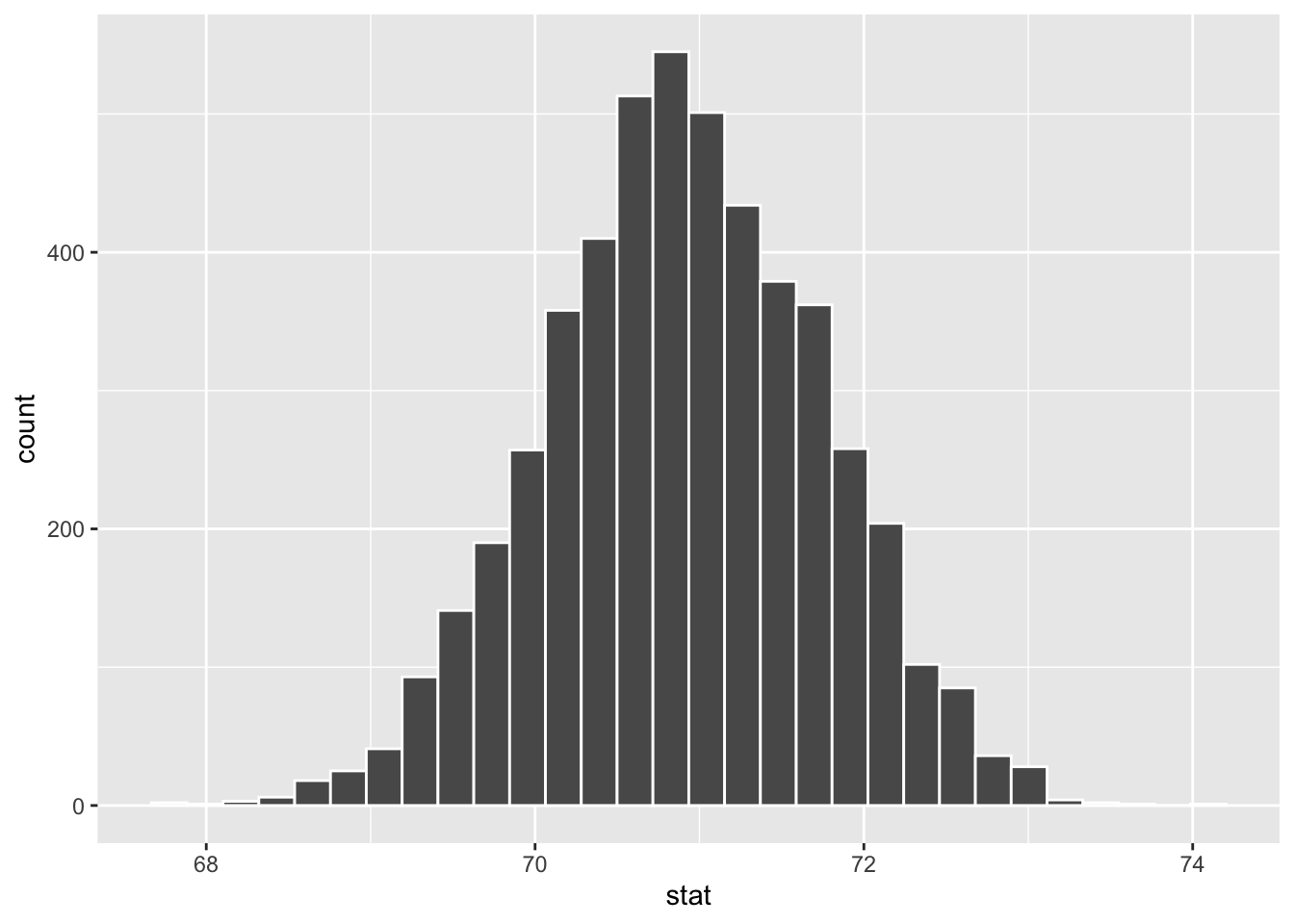idth`.

Although the original data of waiting times was bimodal (from Q6), the bootstrap distribution of the mean becomes unimodal and roughly symmetric. (Although there’s room to quibble - the data aren’t fully symmetric, so if you only picked unimodal, you’re ok!).

This happens because the process of averaging smooths out extremes. Each bootstrap sample contains a mix of high and low waiting times, so the means calculated from them tend to cluster together in the middle. This creates the single, symmetric peak you see here. We will rely on this idea when we explore the normal distribution and the central limit theorem later in the book.

Q9) Following up on the previous question, the lower bound of the 99% confidence interval of mean waiting time is `r

Notice this question asks for a 99% confidence interval. We choose a higher confidence level like this when the consequences of being wrong (i.e., failing to capture the true population mean) are more severe.

This greater confidence comes at a cost, however. A 99% confidence interval is always wider and less precise than a 95% interval calculated from the same data.

Q10) If you were to find the bootstrap standard error you would calculate the ___ of the bootstrap distribution

📊 Glossary of Terms

Bootstrap Distribution: The distribution of a statistic (e.g., the mean) calculated from a large number of bootstrap samples. It’s used to approximate the sampling distribution.
Bootstrap Replicate (or Bootstrap Sample): A new sample of the same size as the original, created by randomly drawing observations from the original sample with replacement.
Bootstrap Standard Error: The standard deviation of the bootstrap distribution, which serves as an estimate of the standard error of an estimate.
Bootstrapping: A computational resampling method that approximates the sampling distribution by repeatedly taking samples with replacement from the original data.
Confidence Interval (CI): A range of plausible values for an unknown population parameter, calculated from sample data. For example, a 95% confidence interval is generated by a process that is expected to capture the true parameter 95% of the time.
Confidence Level: Reasonable bounds we put around our estimate to acknowledge sampling error’s impact on it.
Sampling with Replacement: A sampling process where each selected item is returned to the pool before the next item is drawn, meaning an individual can be selected more than once. This is the core mechanism of bootstrapping.
Sampling without Replacement: A sampling process where a selected item is not returned to the pool, ensuring that all items in the final sample are distinct. This is how traditional statistical samples are taken.

R Packages Introduced

infer: provides a standardized, intuitive framework for performing statistical inference, including bootstrapping.
Hmisc: ggplot2 requires this package to use the mean_cl_boot option within stat_summary(), which automatically calculates and plots bootstrap confidence intervals.

🛠️ Key R Functions

The infer pipeline

specify(): The first step in an infer pipeline, where you declare the variable(s) of interest, using formula syntax like response ~ explanatory.
generate(): The second step, used to create resamples from the data. You specify type = "bootstrap" to generate bootstrap samples.
calculate(): The third step, which computes a summary statistic (e.g., stat = "mean", stat = "diff in means", stat = "slope") for each of the bootstrap replicates.
get_ci(): A convenient final step that calculates a confidence interval from the bootstrap distribution generated by the pipeline.

Other usefull functions

stat_summary(): A powerful function that calculates and plots a summary of your data. In this chapter, it’s used with fun.data = "mean_cl_boot" to automatically perform bootstrapping and plot the mean and confidence interval.
quantile() (stats): Calculates quantiles from a distribution, used to find the lower and upper bounds of a confidence interval.
sd() (stats): Calculates the standard deviation, used to find the standard error from the bootstrap distribution.

Additional resources

Readings:

Resampling-based methods for biologists - J. R. Fieberg et al. (2020).
Chapter 8: Estimation, Confidence Intervals, and Bootstrapping from (Ismay & Kim, 2019).
Chapter 2: Bootstrapping from J. Fieberg (2024).
Chapter 16: Visualizing uncertainty from (Wilke, 2019)

Webapps:

This webapp from Whitlock & Schluter (2020) is great for thinking about confidence intervals. It’s math-based, not bootstrapped-based, but hte concepts and ideas are the same.