• 11. Sampling summary

Links to: Summary. Chatbot tutor. Questions. Glossary. R functions. More resources.
Chapter summary
We almost never know the truth (the population parameter), but we estimate it from a sample. Random chance (aka sampling error) ensures that our estimate will deviate from the true parameter. If sampling error is our only issue we can envision the “sampling distribution” – a histogram of what we would see if we repeated our study many times to characterize uncertainty. We quantify uncertainty as the “standard error” i.e. the standard deviation of the sampling distribution. We can decrease sampling error by increasing sample size. When samples are non-independent, we tend to underestimate our sampling error. When samples are not chosen at random, “sampling bias” can generate a systematic deviation between estimates and true population parameters. Random sampling is our best protection against non-independence and sampling bias.
Chatbot tutor
Please interact with this custom chatbot (link here) I have made to help you with this chapter. I suggest interacting with at least ten back-and-forths to ramp up and then stopping when you feel like you got what you needed from it.
Practice Questions
Try these questions! By using the R environment you can work without leaving this “book”. To help you jump right into thinking and analysis.
Q1) The ___ describes the variability among individual observations in a sample (or population). In other words, the ____ quantifies how far we expect individuals to deviate from the sample estimate. .
Q2) The ___ describes the variability among estimates (of a fixed size) from a population. In other words, the ____ quantifies how far we expect sample estimates to deviate from the population parameter. .
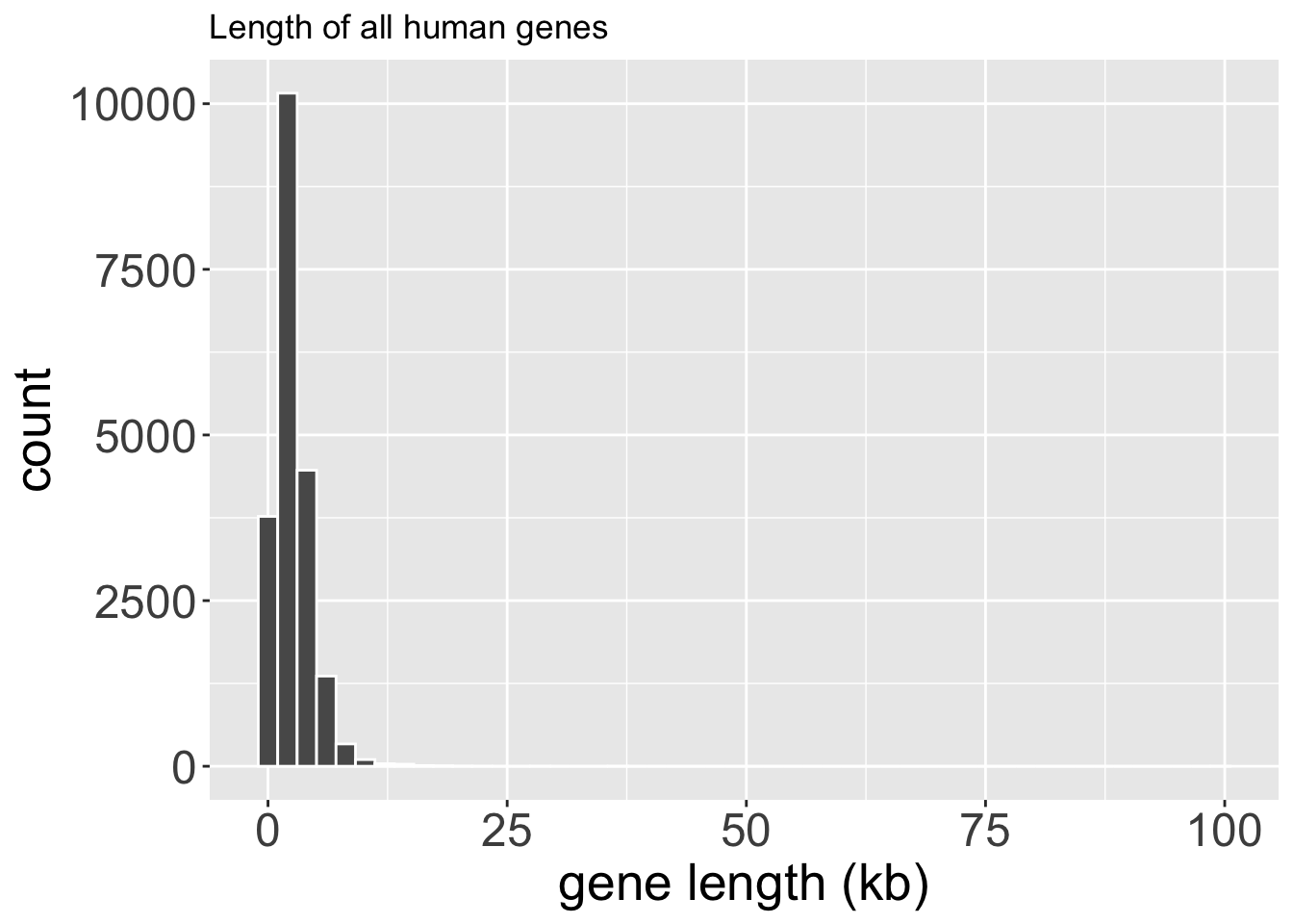
Q3) As seen in Figure 2, the distribution of human gene lengths is ___ (find all correct)
.
Q4) Figure 2 displays ___Sampling wrong: I tried to create a sampling distribution for median human gene length by randomly selecting nucleotides from the human exome, finding the gene they were in, noting its length, and removing it from my list until I had the lengths of fifty genes in the human genome. I did this one thousand times to get medians from one thousand samples of size fifty (Figure 3).
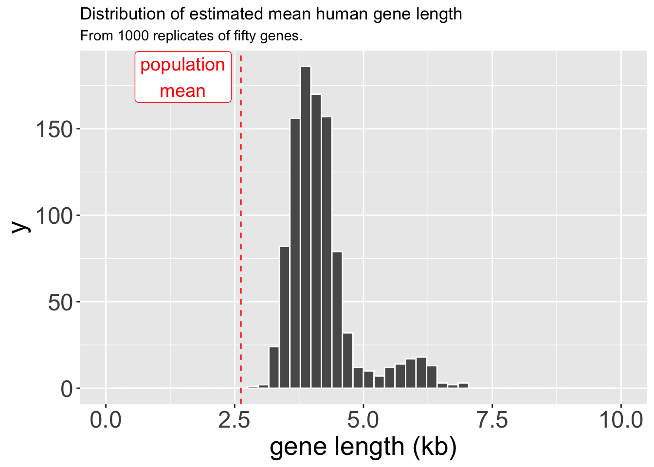
Q5) The difference between the true population mean (red line) and my estimates from samples of size fifty (bars in histogram) are most likely explained by
.
Q6)
Q7) Why is the range of values so much smaller in Figure 3 than in Figure 2?For the following questions, refer to Figure 4 (right).
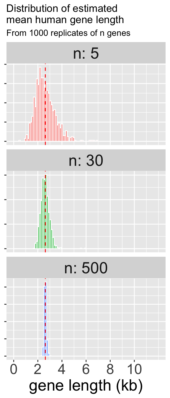
Q8) What aspect of sampling is responsible for the difference between the plots in Figure 4?
Q9) Which sample size is associated with the smallest standard error?
Q10) For the sampling distribution for samples of size n in Figure 4, approximately what proportion samples have a mean greater than the population mean?
- n = 5: .
- n = 500: .
Q11) For the sampling distribution for samples of size n in Figure 4, approximately what proportion samples have a mean greater than 3.8 kb?
- n = 30: .
- n = 500: .
REFRESHER For the questions below summarize the gene lengths data set. If there is not an answer, type NA.
Q12) The mean gene length is .
Q13) The standard deviation in gene length .
Q14) The standard error in estimated gene length .
This is the entire populations. We have a parameter known withoutsampling error, so there is not standard error.
📊 Glossary of Terms
Convenience sampling (aka haphazard sampling): Sampling whatever is easiest or closest.
Independent sample A sample where knowing something about one observation tells you nothing about the others.
Non-independent sample A sample where some observations are related to each other. This messes with your uncertainty estimates unless accounted for.
Parameter: A number that describes the truth about a population (e.g. the actual mean petal area of all Clarkia xantiana plants on Earth).
Pseudoreplication: Using repeated but non-independent measurements as if they were independent. This can lead to overconfidence and misleading results.
Random sample: A sample where each individual has an equal chance of being selected.
Sampling: Selecting a subset of individuals from a population.
Sampling Bias: Any process that causes a sample to be systematically unrepresentative of the population.
Sampling Distribution: A histogram of what you’d get if you repeated your study over and over, taking a new sample each time and recording the resulting estimate.
Sampling Error: The random difference between an estimate from a sample and the true population parameter.
Standard Error (SE): The standard deviation of the sampling distribution. Measures the expected variability in your estimates due to sampling error.
Survivorship bias: A kind of sampling bias where you only observe individuals that survive some process (e.g., returning warplanes), which can give a misleading picture of the whole population.
Key R Functions
sample(): Samples values from a vector.
slice_sample()(dplyr): Samples rows from a tibble.
Additional resources
Readings:
Module: Standard Error from Teacups Giraffes and Statistics, by Hasse Walum and Desirée De Leon.
Chapter 7 Sampling from (Ismay & Kim, 2019).
Pages 104-112 and 126-133 about sampling bias from Bergstrom & West (2020).
Interleaf 2: Pseudo-replication from Whitlock & Schluter (2020).