library(ggplot2)
library(palmerpenguins)

# The base plot we will improve upon
base_plot <- ggplot(penguins, aes(x = species, y = flipper_length_mm)) +
  geom_point()

base_plot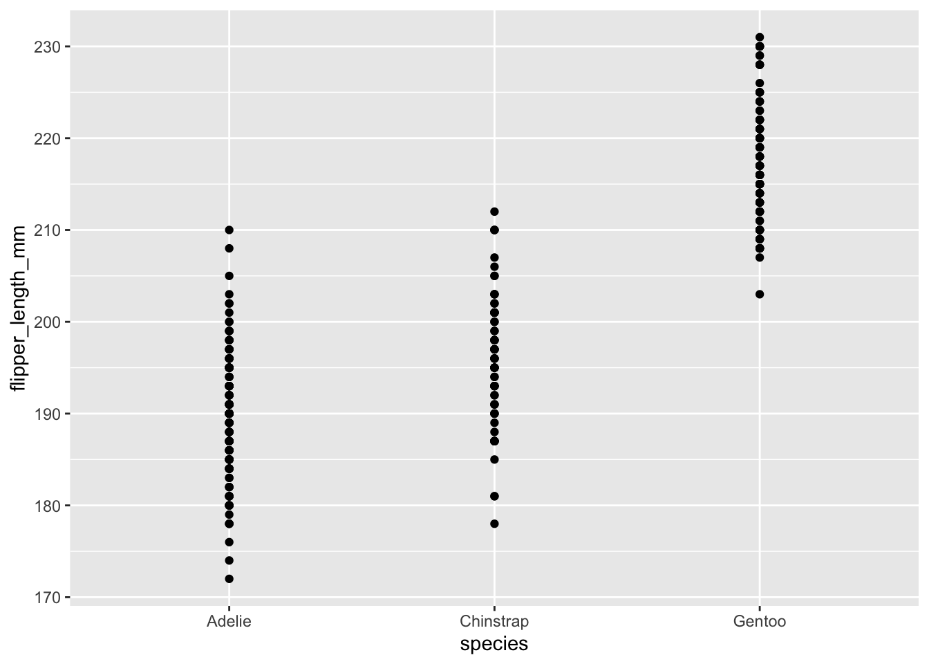
Links to: Summary. Chatbot tutor. Questions. Glossary. R functions. R packages. More resources.
Polishing a ggplot plot is not about running a single command, but is an iterative process of refinement, moving from a default chart to a polished, explanatory figure.
We do this by layering components. We start with a basic plot and add functions to clarify labels (with the labs() function and the ggtext package) and control aesthetics like color and shape (with scale_*_manual()). We then adjust non-data elements with the theme() function, arrange categories logically with the forcats package, and combine plots into larger narratives with patchwork.
Throughout this process, we also make sure to consider the presentation format, tailoring our choices for each specific medium. A working understaing of ggplot is essential, but luckily you don’t need to have all this memorized—knowing how to use books, friends, chatbots, GUIs like ggThemeAssist, and other resources can help!
Please interact with this custom chatbot (link here) I have made to help you with this chapter. I suggest interacting with at least ten back-and-forths to ramp up and then stopping when you feel like you got what you needed from it.
The following questions will walk you through the iterative process of refining a plot, from a messy default to a polished, clear visualization.
To start, let’s create a basic plot from the palmerpenguins dataset. It shows the distribution of flipper lengths for each species. As you can see, it has several problems we need to fix!
library(ggplot2)
library(palmerpenguins)
# The base plot we will improve upon
base_plot <- ggplot(penguins, aes(x = species, y = flipper_length_mm)) +
geom_point()
base_plotQ1) The plot above suffers from severe overplotting, making it hard to see the distribution of points. Which geom_* function is specifically designed to fix this by adding a small amount of random noise to the points’ positions?
Q2) Let’s fix the overplotting. In the R chunk below, replace geom_point() with the correct function from the previous question. To keep the data honest, make sure all y-values stay the same, and that x values are clearly associated with a category.
In the geom_*_ Set the height argument to 0 and providing a small width (e.g., 0.2)
Q3) Great! Now look at the x-axis. ggplot2 defaults to alphabetical order (Adelie, Chinstrap, Gentoo). Use fct_reorder() from the forcats package to reorder the species factor from largest to smallest median flipper length. Now which species now appears first (leftmost) on the x-axis?
Add a mutate() call before ggplot()
Add a .na_rm =TRUE to ignore NA values and .desc = TRUE to go from greatest to smallest.
library(forcats)

penguins |>
  mutate(species = fct_reorder(species, flipper_length_mm, median, .na_rm =TRUE, .desc = TRUE))|>
  ggplot(aes(x = species, y = flipper_length_mm)) +
  geom_jitter(width = 0.2, height = 0)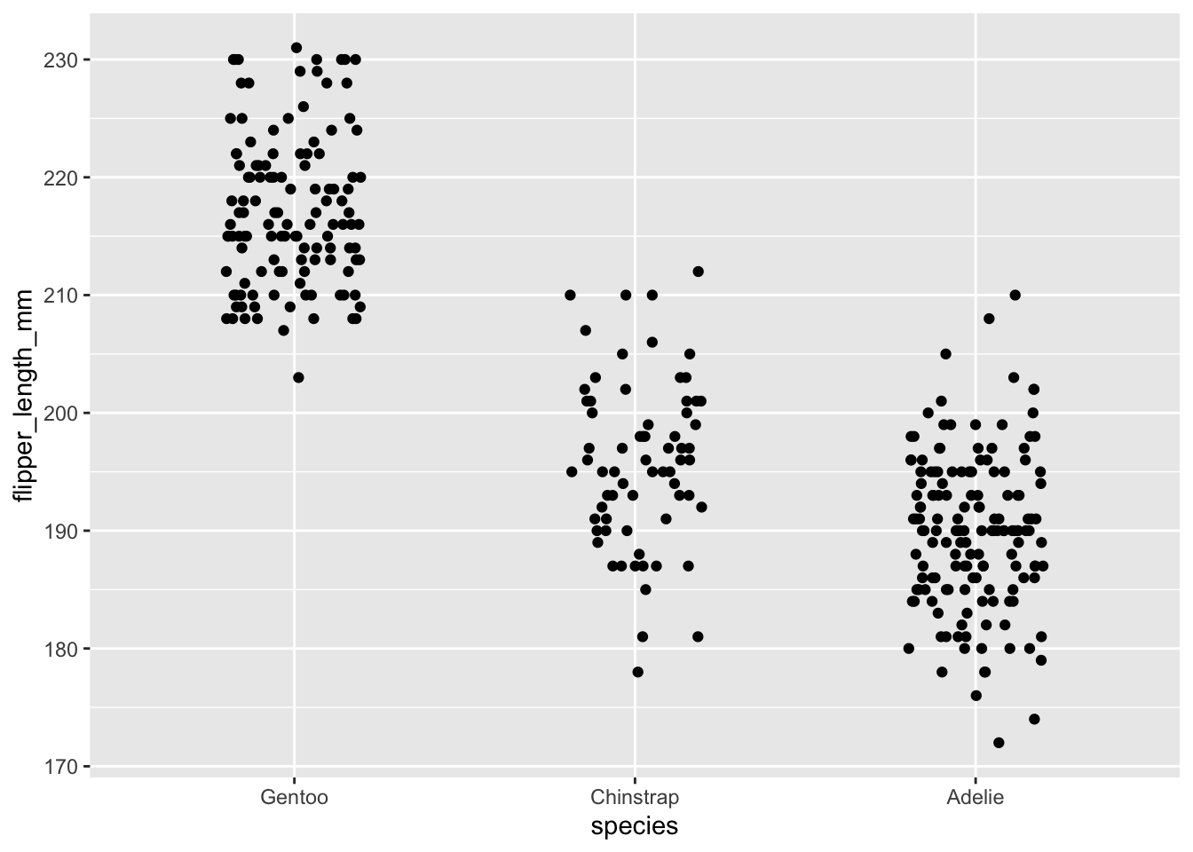
Q4) Our plot is now well-organized, but the labels are not publication-ready. Add a labs() layer to the good_start plot above to achieve the following:
title to “Penguin Flipper Lengths”x axis label to “Species”y axis label to “Flipper Length (mm)”The labs() function is used to change titles and axis labels. If you also wanted to change the title of the color legend, which argument would you add inside labs()?
Q5) Now, imagine you need to put this plot on a slide for a presentation. The text is far too small. Add a theme() layer to the code below to make the axis titles (axis.title) size 20.
Inside theme(), the element_text() function has many arguments besides size. Which argument would you use to change the font from normal to bold?
Q8) The plot above shows the raw data well. Now, let’s add a summary statistic. In the webr chunk below, add a stat_summary() layer to display the mean value for each species as a large, black point (size = 5, color = "black"). Hint: You’ll need to specify fun = "mean" and geom = "point" inside stat_summary().
Q9) Faceting is a powerful way to create “small multiples.” In the chunk above, add a facet_wrap() layer to the scatter plot to create separate panels for each island.
After adding the facet layer correctly, which Islands have Chinstrap penguins? (select all correct)
color and shape). This improves clarity and accessibility.*All functions are in the ggplot2 package unless otherwise stated.
geom_image() ([ggimage]): Adds images to a plot, often used to represent data points or summaries.labs(): The primary function for setting the plot’s title, subtitle, caption, and the labels for each axis and legend.
geom_label() / geom_text(): Adds text-based labels to a plot, mapping data variables to the label aesthetic. geom_label() adds a background box to the text.
annotate(): Adds a single, “one-off” annotation (like a piece of text or a rectangle) to a plot at specific, manually-defined coordinates.
element_markdown() In the ggtext package: Used inside theme() to render plot text (like axis labels or facet titles) that contains Markdown or HTML for styling.
stat_summary(): Calculates summary statistics (like means or confidence intervals) on the fly and adds them to the plot as a new layer (e.g., as bars or errorbars). This in gplot2, but required the Hmisc package.
fct_reorder() In the forcats package: Reorders the levels of a categorical variable (a factor) based on a summary of another variable (e.g., order sites by their mean petal area).
fct_relevel() In the forcats package: Reorders the levels of a factor “by hand” into a specific, manually-defined order.
scale_color_manual() / scale_fill_manual(): Manually sets the specific colors or fill colors for each level of a categorical variable.
scale_color_brewer() / scale_fill_brewer(): Applies pre-made, high-quality color palettes from the RColorBrewer package.
scale_color_viridis_d() / scale_color_viridis_c(): Applies perceptually uniform and colorblind-friendly palettes from viridis. Use _d for discrete data and _c for continuous data.
facet_wrap(): Creates “small multiples” by splitting a plot into a series of panels based on the levels of a categorical variable.
plot_annotation() In the forcats package: Adds overall titles and panel tags (e.g., A, B, C) to a combined figure.
plot_layout() In the forcats package: Controls the layout of a combined figure, such as collecting all legends into a single area.
theme(): The master function for modifying all non-data elements of the plot, such as backgrounds, grid lines, and text styles.
element_text(): Used inside theme() to specify the properties of text elements, like size, color, and face (e.g., “bold”).
theme_classic() / theme_bw(): Applies a complete, pre-made theme to a plot with a single command, often for a cleaner, publication-ready look.
ggplot2: The core package we use for all plotting, based on the Grammar of Graphics.
dplyr: Used for data manipulation and wrangling, like filter() and mutate().
forcats: The essential tool for working with categorical variables (factors), especially for reordering them in a logical way.
patchwork: A tool for combining separate ggplot objects into a single, multi-panel figure.
ggtext: A powerful package that allows you to use rich text formatting (like Markdown and HTML) in plot labels for effects like italics and custom colors.
Hmisc: A general-purpose package that contains many useful functions, including mean_cl_normal for calculating confidence intervals in stat_summary().
scales: Provides tools for controlling the formatting of numbers and labels on plot axes and legends.
ggimage: Used to add images as data points or layers in your plots.
ggtextures: Allows you to create isotype plots (bar graphs made of images).
gganimate: Brings your static ggplots to life by creating animations.
[ggthemes]https://github.com/jrnold/ggthemes): Provides a collection of additional plot themes, including styles from publications like The Economist and The Wall Street Journal.
plotly: A powerful package for creating interactive web-based graphics. Its ggplotly() function can make almost any ggplot interactive with one line of code.
highcharter: Another popular and powerful package for creating a wide variety of interactive charts.
Shiny: R’s framework for building full, interactive web applications and dashboards directly from your R code.
MetBrewer: Provides beautiful and accessible color palettes inspired by artworks from the Metropolitan Museum of Art.
wesanderson: A fun package that provides color palettes inspired by the films of director Wes Anderson.
ggThemeAssist: An RStudio add-in that provides a graphical user interface (GUI) for editing theme() elements, helping you learn how to customize your plot’s appearance.Interactive Cookbooks & Galleries:
The R Graph Gallery: An extensive, searchable gallery of almost every chart type imaginable, created with ggplot2 and other R tools. Each example comes with the full, reproducible R code.
From Data to Viz: A fantastic tool that helps you choose the right type of plot for your data. It provides a decision tree that leads to ggplot2 code for each chart.
The ggplot2 Extensions Gallery: The official showcase of packages that extend the power of ggplot2 with new geoms, themes, and capabilities. A goodt place to discover new visualization tools in the R ecosystem.
A ggplot2 Tutorial for Beautiful Plotting in R Many fantastic examples. This is great! Have a look!
Online Books:
R Graphics Cookbook, 2nd Edition: A great “how-to” manual by Winston Chang. It is a collection of practical, problem-oriented “recipes” for solving common plotting tasks in ggplot2.
Data Visualization: A Practical Introduction: Kieran Healy’s blends data visualization theory with practical ggplot2 code.
Interactive web-based data visualization with R, plotly, and shiny: A guide by Carson Sievert for turning your ggplot2 plots into interactive graphics and building web applications. This is a bit dated, but still useful.
Data Visualization with R: A fantastic course on data visualization by Andrew Heiss.
Videos & Community:
The #TidyTuesday Project: A weekly data project from the R for Data Science community. It is the best place to see hundreds of creative and inspiring examples of what’s possible with ggplot2 and to practice your own skills.
Data visualization with R’s tidyverse and allied packages A collection of videos by Pat Schloss includes maps, community microbiolgy and more.