• 19. ANOVA: a linear model

Motivating Scenario: You know that many statistical models are simply a type of linear model. How can we think about an ANOVA as a linear model and intrpret the coefficients from thsi model

Learning Goals: By the end of this subchapter, you should be able to:

Recognize that ANOVA is a special case of a linear model.
Interpret model coefficients (intercept, slopes) in the context of group means.
Know what a residual is and find residual values with math or the augment() function.
Change the reference level and interpret how it affects model output.

Recall that “linear models” are “linear” because we find an individual’s predicted value \(\hat{Y_i}\) by adding up predictions from each component of the model. So, for example, \(\hat{Y_i}\) equals the parameter estimate for the “intercept”, \(a\), plus its value for the first explanatory variable, \(y_{1,i}\), times the effect of this variable, \(b_1\), plus its value for the second explanatory variable, \(y_{2,i}\) times its effect, \(b_2\), etc.

\[\hat{Y}_i = a + b_1 y_{1,i} + b_2 y_{2,i} + \dots{}\]

Just like a one or two sample t-test, the ANOVA is a linear model. As such, it models group means as a function of group membership. This works by picking one group as the “reference level” and having that group’s mean represented as the intercept. Then each “slope” \(b\) is the difference between that group’s mean and the reference group’s mean, and the corresponding \(y_i\)s are one if the individual is in that group and zero otherwise.

By default R chooses the reference levels as the alphabetically first one. We often don’t want that (e.g. you may want the control to be first). The fct_relevel() function in the forcats package can help (see fyi below)!

hybrid_anova <- lm(admix_proportion ~ site, data = clarkia_hz )

(Intercept)     siteS22      siteSM      siteS6 
     0.0071      0.0183      0.0025      0.0221

We cast this as a linear model as follows: \(\widehat{\text{admix prop}}_i = 0.0071 + 0.0183 \times \text{S22}_{i} + 0.0025 \times \text{SM}_{i} + 0.0221 \times \text{S26}_{i}\).

Here SR is the “reference level”, and as such, SR’s mean admixture proportion equals the intercept, 0.0071. Similarly, we estimate an admixture proportion of 0.0183 + 0.0071 = 0.0254 at site S22.

Your turn: Use the linear model output to find the estimated admixture proportion at each of the following locations:

Squirrel Mountain(SM) .
Site 6 (S6) .

Residuals

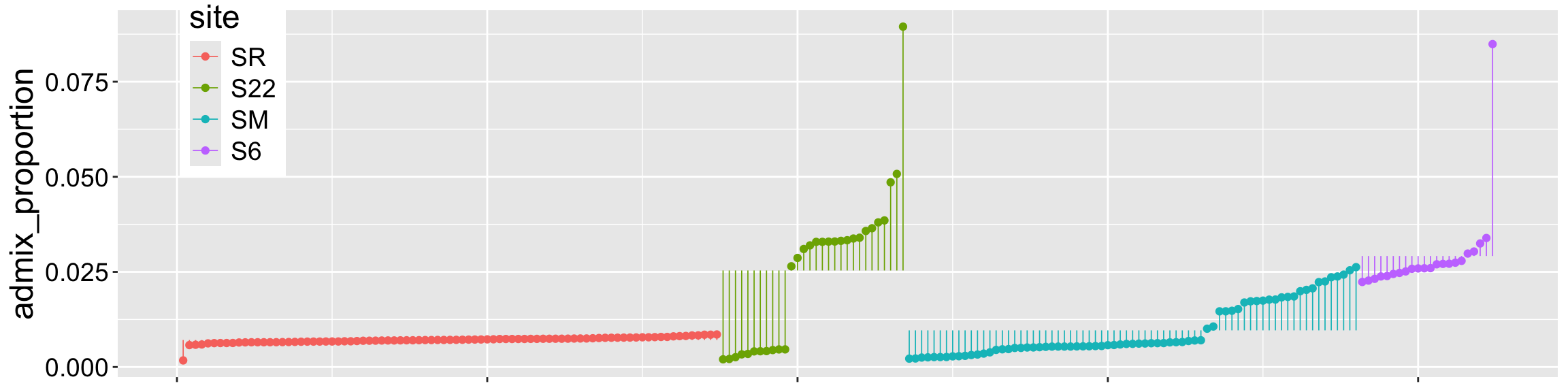
Of course, individual observations deviate from their predicted value! As you know by now the difference between an observation, \(Y_i\) and its predicted value, \(\hat{Y_i}\) is called the residual, \(\epsilon_i\). Figure 1 shows the residuals as the length of the lines connecting individual observations to group means.

Mathematical descriptions of residuals \[\hat{Y_i}=Y_i+\epsilon_i\] \[Y_i=\hat{Y_i}-\epsilon_i\] \[\epsilon_i= Y_i-\hat{Y_i}\]

Recall that the augment() function in the broom package shows \(\hat{Y_i}\) as the .fitted column, and the residuals as the .resid column:

library(broom)
augment(hybrid_anova)

admix_proportion	site	.fitted	.resid
0.0265	S22	0.0254	0.0011
0.0329	S22	0.0254	0.0075
0.0895	S22	0.0254	0.0641
0.0042	S22	0.0254	-0.0212
0.0041	S22	0.0254	-0.0212
0.0033	S22	0.0254	-0.0221

Changing reference levels Alphabetical order is not always the “right” order. For example, in this data set of Daphnia resistance to a poisonous cyanobacteria across years with high, medium and low concentrations of cyanobacteria.

daphnia_data <- read_csv("https://whitlockschluter3e.zoology.ubc.ca/Data/chapter15/chap15q17DaphniaResistance.csv")

lm(resistance ~ cyandensity, data = daphnia_data)


Call:
lm(formula = resistance ~ cyandensity, data = daphnia_data)

Coefficients:
   (Intercept)  cyandensitylow  cyandensitymed  
        0.8000         -0.1167         -0.0170

The code below uses the fct_relevel() function in the forcats package to change the order of our factors, so the reference level makes more sense.

library(forcats)
daphnia_data <- daphnia_data |>
  mutate(cyandensity =fct_relevel(cyandensity, "low","med","high"))

lm(resistance ~ cyandensity, data = daphnia_data)


Call:
lm(formula = resistance ~ cyandensity, data = daphnia_data)

Coefficients:
    (Intercept)   cyandensitymed  cyandensityhigh  
        0.68333          0.09967          0.11667