• 15. Normal Properties

Motivating scenario: You’re brushing up on your understanding of the normal distribution.

Learning goals: By the end of this chapter you should be able to:

List the key properties of a normal distribution.
Use an interactive tool to find the probability of a random value falling within a specific range of the Standard Normal Distribution.
Apply the Addition and Complement rules of probability to calculate the probability of combined events.
Explain a Z-score and how to change any normal distirbution into the standard normal distribution.

Now that we have the basics of the normal distribution down, let’s consider some of its properties. While I don’t believe in “making” students memorize anything, these are basic facts that anyone who deals with statistics should be pretty comfortable with:

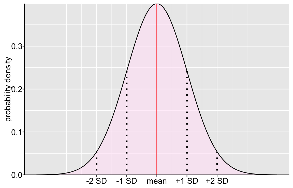
The normal distribution is symmetric about its mean. This means that if you folded a paper with the normal distribution printed on it, and folded it in half (with the fold centered on the mean), one side would lay perfectly atop the other.
\(50\%\) of the normal distribution is less than its mean.
\(50\%\) of the normal distribution is greater than its mean.
\(\approx 68\%\) of the normal distribution is within one standard deviation of the mean.
\(\approx 95\%\) of the normal distribution is within two standard deviation of the mean.

We briefly go over these properties below. As we do so, we will also review some basic probability theory.

A diagram of a normal distribution curve. A symmetric, bell-shaped curve is plotted with "probability density" on the y-axis. The x-axis is marked at the "mean", and at intervals of "+1 SD", "-1 SD", "+2 SD", and "-2 SD". A vertical red line indicates the mean, and dotted black lines extend down from the curve at each standard deviation mark. The area under the curve is shaded light pink. — Figure 1: The probability density function (PDF) of a generic normal distribution. The curve is symmetric with its peak at the mean (μ), and the horizontal axis is marked in units of standard deviation (σ).

Exploring Probabilities with the Standard Normal Distribution

These properties are true for any normal distribution, regardless of its mean or standard deviation. But to make them concrete, let’s start with a normal distribution with a mean of zero and a standard deviation of one. This is known as the Standard Normal Distribution. The standard normal is convenient because the values on the x-axis (like -2, -1, 1, 2) directly correspond to the number of standard deviations from the mean.

We can dust off our integral calculus to find the probability that a value of X falls within a range (see the margin). But if you (like me) would rather use a computer and simple arithmetic we can avoid calculus! I have created a webapp (below) to help get started with these ideas, after a bit of practice with the webapp, I’ll introduce some probability theory rules to help combine probabilities.

We can find the probability that X lies between two values, \(a\) and \(b\), by finding the integral of the normal curve from a to b as follows.

\[P[a < X < b] = \int_{a}^{b} \frac{1}{\sqrt{2\pi \sigma ^{2}}}e^{-\frac{(x-\mu) ^{2}}{2\sigma ^{2}}} dx\]

Now let’s play with this webapp to get more intuition for the normal distribution!

To see that the normal distribution is symmetric around its mean:
- Drag the cursor from 0 to the right tail (i.e. past four), and then from 0 to the left tail (i.e. past negative four). Both values should be 0.5.
- Drag the cursor from 1 to its right tail, and then from -1 to its left tail. Both values should be 0.1586.
- Drag the cursor from 2 to its right tail, and then from -2 to its left tail. Both values should be 0.0227.
To see that the \(\approx 68\%\) of the normal distribution is within \(\sigma\) of the mean:
- Drag the cursor from -1 to 1. You should get about 0.683.
To see that the \(\approx 68\%\) of the normal distribution is within \(2\times \sigma\) of the mean:
- Drag the cursor from -2 to 2. You should get about 0.955.

Practice What is the probability that a random draw from a normal distribution is between one and one and a half standard deviations greater than the mean? .

You can solve this in one step with the web app! Click your mouse at x = 1 and drag it to x = 1.5 to find the area between them.

The Z-Transformation

The web app is a great tool for understanding the standard normal distribution. But how does this help us with our flower data, which has a mean of 1.7815 and a standard deviation of 0.0998?

The answer is a powerful tool called the Z-transformation. It’s a simple formula that allows us to convert any value from any normal distribution into an equivalent value on the standard normal distribution. This means we can solve any normal distribution problem by converting it to the standard normal first.

We z-transform data by taking each value, subtracting the mean, and dividing by the standard deviation. So, if the \(i^{th}\) observation has a value of \(x_i\), its z-value is:

\[z_i=\frac{x_i-\mu}{\sigma}\]

So, although we just worked through the results thinking about the standard normal, they apply to any normal distribution!

The mathematical notation for a normal distribution is written as follows:

\[X \sim \mathcal{N}(\mu,\,\sigma^{2})\]

So the standard normal is written as: \(X \sim \mathcal{N}(0,\,1^2)\).
And a normal with a mean of \(1.78\), and an sd of 0.1 (i.e. a variance of \(0.01\)) is written as: \(X \sim \mathcal{N}(1.78,\,0.01)\).