• 15. Normal Introduction

Motivation: You are getting ready to conquer the normal distribution and just need to set a few things in place.

Learning goals: By the end of this chapter you should be able to:

1. Identify the key features of a normal distribution and its parameters:

   • The center: Mean (\(\mu\)).
     
   • The width: Standard deviation (\(\sigma\)).

2. Explain the concept of a probability density for continuous data and how it differs from a probability mass function for discrete data.

3. Use R’s dnorm() function to find the probability density of a specific value from a normal distribution.
   

4. Know that the standard error is the the standard deviation of the sampling distribution.

   • The standard error of a sample from a normal distribution is \(\sigma/\sqrt{n}\) where \(n\) is the sample size.
     

---

A normal-ish distribution

gc_rils <- gc_rils|> 
  mutate(log10_petal_area_mm = log10(petal_area_mm))

gc_rils_summaries <- gc_rils  |> 
  summarise(mean_log10_petal_area = mean(log10_petal_area_mm, na.rm = TRUE),
            sd_log10_petal_area   = sd(log10_petal_area_mm, na.rm = TRUE))

gc_rils_mean_log10_petal_area <- pull(gc_rils_summaries, mean_log10_petal_area)
gc_rils_sd_log10_petal_area <- pull(gc_rils_summaries, sd_log10_petal_area)
this_n <- gc_rils |> summarise(n = sum(!is.na(petal_area_mm))) |> pull()

gc_rils_mean_log10_petal_area <- pull(gc_rils_summaries, mean_log10_petal_area)
gc_rils_sd_log10_petal_area <- pull(gc_rils_summaries, sd_log10_petal_area)
this_n <- gc_rils |> summarise(n = sum(!is.na(petal_area_mm))) |> pull()

ggplot(gc_rils, aes(x = log10_petal_area_mm))+
    geom_histogram(color = "white", binwidth = .06)+
    stat_function(fun = function(x) { 
       this_n * .06 * dnorm(x,
                           mean = gc_rils_mean_log10_petal_area ,
                           sd = gc_rils_sd_log10_petal_area) },
      color = "red", linewidth = 1, xlim = c(1.45,2.1))+
  labs(x = expression(paste("log"[10], " petal area (mm)")),
       y = "count")+
  theme(axis.title = element_text(size = 16),
        axis.text = element_text(size = 16))

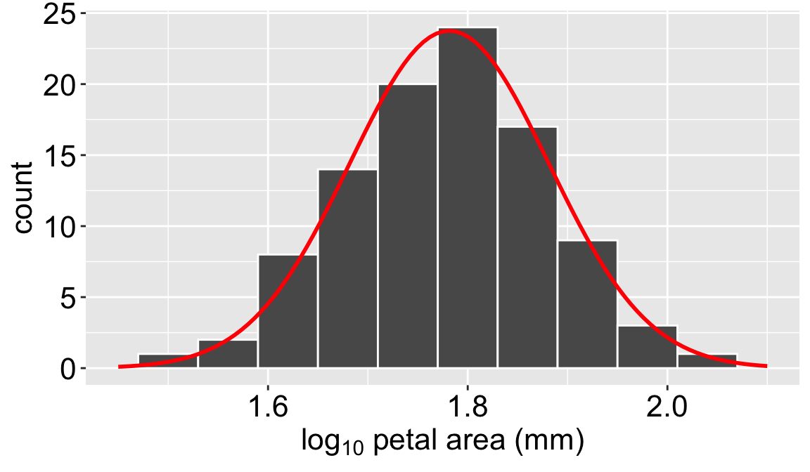
Figure 1: A histogram showing the distribution of the log_10 transformed petal area. The red line shows the theoretical normal distribution with the same mean and standard deviation as the sample.

Petal areas (even after being log transformed) aren’t perfectly normal, but they are close enough that the normal distribution is a useful approximation. Remembering that all models are wrong, but some are useful is key. Stats relies on useful but imperfect models - and it is our job as statisticians to recognize when a model is good enough and when it is downright inappropriate.

To see what this looks like in practice, let’s compare our flower data to a normal distribution fit by parameter estimates from our data. The similar shape of the histogram and the normal distribution plotted over it (in red), demonstrates that the \(log_{10}\)-transformed petal area of parviflora RILs (Figure 1) planted at GC is well-approximated by a normal distribution (with mean, \(\bar{x}\) = 1.7815, and sd, s = 0.0998). We will therefore start with this example to understand properties of a normal distribution while picking up some probability theory and R tricks along the way.

mean	sd
1.7815	0.0998

g_petal_summaries <- gc_rils  |> 
  summarise(mean = mean(log10_petal_area_mm, na.rm = TRUE),
            sd   = sd(log10_petal_area_mm, na.rm = TRUE))

---

For the rest of this section we will deal with a population with a mean \(\mu\) of 1.7815, and a standard deviation, \(\sigma\) of 0.0998, rather than our sample. Note that I have gone back and forth on if I write mean and standard deviation with an English or Greek symbol… there is a method to the madness:

• Greek letters like \(\mu\) and \(\sigma\) refer to population parameters.
  
• English symbols (typically \(\bar{x}\) for mean, and \(s\) for the standard deviation), refer to sample estimates.

---

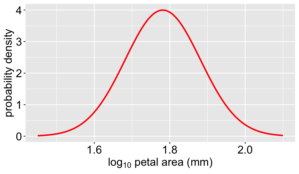
Probability density functions

Figure 2: The normal distribution that fits the log-10 transformed petal area data. The curve shows the probability density for any given value, pretending our sample means and standard deviations where actually parameters in a normal distribution. This raw probability density is proportional to the line in Figure 1, above, but is not scaled to match our sample size or the bin width of the histogram.

Continuous distributions are a bit funny:

• The probability of any particular number (evaluate to infinite digits) is zero
  
• But some observations would be more surprising than others
  • A flower a \(log_{10}\)-transformed petal area of 99 would shock me.
    
  • A flower a \(log_{10}\)-transformed petal area of 1.873892 would be less surprising.

To address this we work, not with raw probabilities, but with probability densities – numbers that are proportional to a probability. The probability density of the Gaussian (aka normal) distribution is equals

\[f(x) = \frac{1}{\sigma\sqrt{2\pi}} e^{-\frac{1}{2}\left(\frac{x-\mu}{\sigma}\right)^2}\]

Note You can use R’s dnorm() function to plug numbers into the Gaussian function for you! The d is for density and the norm is for normal!

So, the probability density of a flower with an area of 1.873892 is
\[f(x) = \frac{1}{0.0998\sqrt{2\pi}} e^{-\frac{1}{2}\left(\frac{1.873892- 1.7815}{0.0998}\right)^2} = 2.604\]

value   <- 1.873892
my_mean <- 1.7815
my_sd   <- 0.0998
dnorm(x     =  value, 
      mean  =  my_mean, 
      sd    =  my_sd)

[1] 2.604191

This means that rather than summing to one (as traditional “probability masses” for categorical or discrete variables do) the probability density integrates to one. Thus, unlike probability masses, probabilities densities (like the one above, and many points in Figure 2) can exceed one.

The Probability Density of a Sample Mean

Remember that the standard deviation of the sampling distribution is called the standard error. To calculate the probability density of a sample mean, we substitute \(\sigma\) (the variance of the normal distribution) with the the standard deviation of a normal distribution (i.e. the standard error of the mean. Mathematically, the standard error of the mean of a normal sampling distribution, \(\sigma_\bar{x}\), equals:

\[\sigma_\bar{x}=\frac{\sigma}{\sqrt{n}}\]

For instance: the probability density that a random draw of size n from a normal distribution with mean 1.7815 of and sd of 0.0998 will have a sample mean of 1.8739 equals:

• dnorm(1.8739, mean = 1.7815, sd = 0.0998/sqrt(2)) = 2.399 for \(n\) of 2.

• dnorm(1.8739, mean = 1.7815, sd = 0.0998/sqrt(10)) = 0.174 for \(n\) of 10.

---

I did some sneaky stuff above, and I want you to think about it for a minute.

Note that I said “the \(log_{10}\)-transformed petal area of parviflora RILs (Figure 1) planted at GC is well-approximated by a normal distribution (with mean = 1.7815, and sd = 0.0998)”.

This is a mathematical approximation, not the true description of this population for two reasons.

1. The values of \(\mu\) and \(\sigma\) are estimates from the sample, not the true parameters.

2. Petal area is not generated by a normal distribution - it is generated by genes, sunlight, nutrients and the like, so the word “approximated” is doing a lot of work here. This is the difference between a mathematical and phenomenological model.

3. Putting aside the concern above - the mathematical description of the data as normal may not be quite right - to my eye the data are somewhat skewed.

But as long as we keep these caveats in our head using the normal distirbution to approximate these data is incredibly useful!