16. The t distribution
Motivating scenario: We just learned about the normal distribution and Z-tests, but we realized a problem - we have a sample not a population. This means we can estimate the mean as \(\bar{x}\) and the standard deviation as \(s\), but we don’t know their true parameter values \(\mu\) and \(\sigma\) (that’s why we’re doing stats after all). What to do? We can turn to the t-distribution!!
Learning goals: By the end of this chapter you should be able to:
Explain the difference between the standard normal distribution (\(Z\)) and the \(t\) distribution.
Interpret a \(t\) value simply.
Calculate and interpret Cohen’s D as a measure of effect size.
Use the \(t\) distribution to calculate a 95% confidence interval for a sample from the normal distribution.
Test the null hypothesis that a sample mean comes from a population with a given parameter value by
- Performing a one-sample t-test.
- Performing a paired t-test.
Use the
_t()family of functions in R to:Use the
t.test()function to conduct one sample and paired t-tests in R.
The Dilemma
- For a single observation, \(z = \frac{x - \mu}{\sigma}\).
- For the mean of a sample of size \(n\), \(Z = \frac{\overline{x} - \mu_0}{\sigma / \sqrt{n}}\).
This allowed us to summarize the distance between an estimated mean, \(\bar{x}\), and its null value, \(\mu_0\), in standardized units (standard errors), regardless of the mean and variance. This is super useful, because e.g. we can conduct null hypothesis significance testing and the like.
However, there’s a problem: We usually have only a sample and not the whole population (that’s why we’re doing statistics after all!). So have an estimate of the standard deviation \(s\), and not its true parameter value \(\sigma\). This means our standard error, too, is an estimate associated with uncertainty. Unfortunately, the Z-distribution does not account for this additional uncertainty.
The Solution
Don’t despair! The t-distribution can rescue us!!!
- Like the standard normal (“Z”) distribution, the t-distribution is unimodal and symmetric.
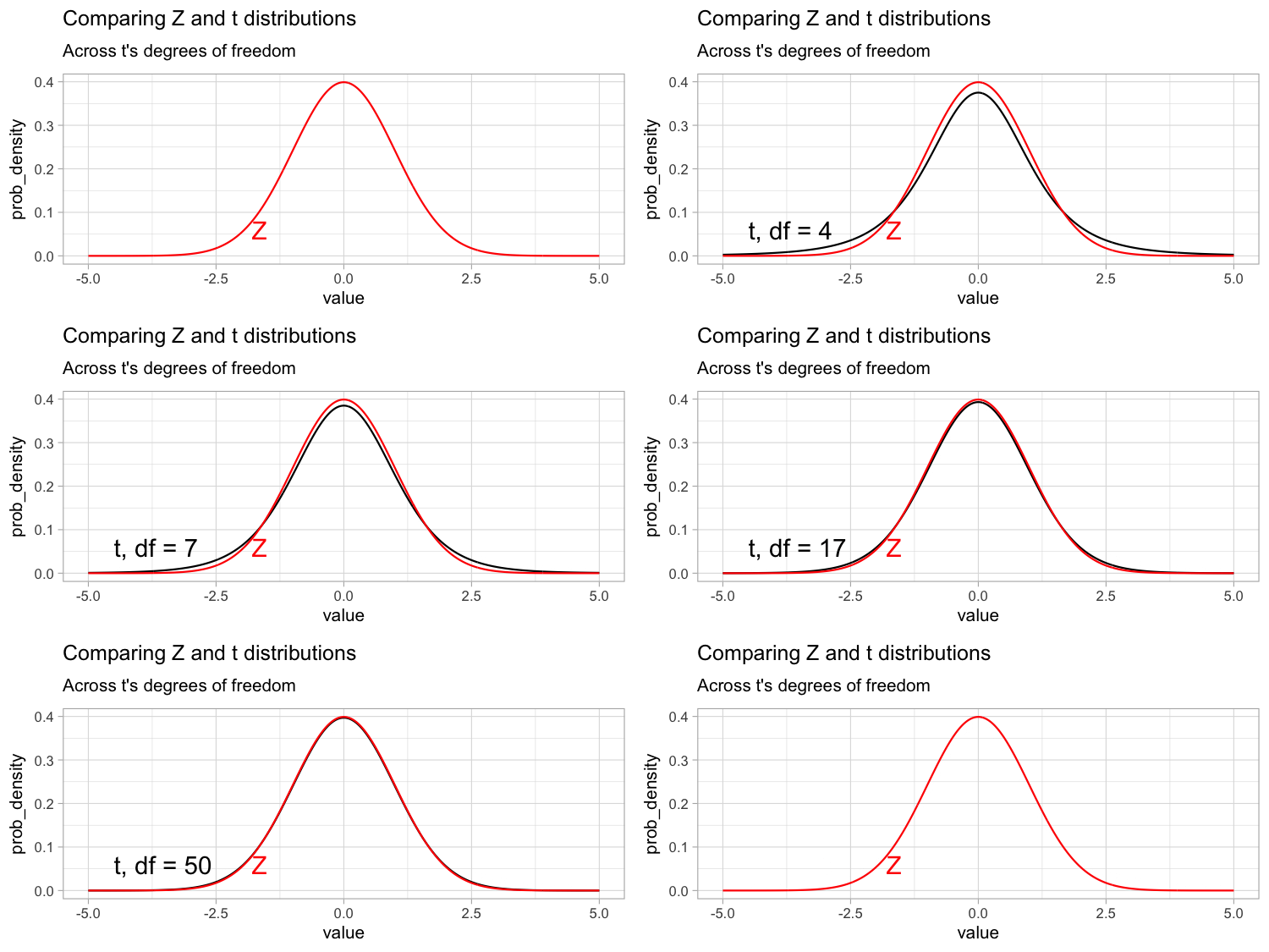
- But, to account for the additional uncertainty that comes from using the sample standard deviation (\(s\)) instead of the true population value (\(\sigma\)), the t-distribution has “fatter tails” than the Z distribution.
Because the tails are “fatter”, a larger proportion of its area in the tails beyond \(\pm2\) (greater than 4.55%, compared to exactly 4.55% for the Z-distribution).
Degrees of freedom

Now you might be wondering:
- How “fat” are the tails of the t-distribution? and
- What proportion of samples from a t-distribution are more than two standard errors away from the population mean?
The answers to these questions depend on which t-distribution we’re talking about. There are many each associated with a certain number of degrees of freedom.
The degrees of freedom reflect the number of observations that can vary before all values are determined, which is related to our uncertainty in our estimate – the more the degrees of freedom, the less uncertainty! As such, tails get less “fat” and the t-distribution looks more and more like the standard normal (z) distribution as the degrees of freedom increase (Figure 1).
t as a Common Test Statistic
Since most sampling distributions are normal, but we rarely know the true population standard deviation, t-values are common in applied statistics. Each time we encounter a t-value, it tells us how many standard errors our estimate is away from the hypothesized parameter under the null hypothesis.
Put simply t is the distance (in standard errors) between our estimate and its proposed value under the null (incorporating uncertainty in our estimate of the standard deviation)
You may see Z-tests in the literature. Z tests are never the “right” thing to do, because we never have a population, but in some cases they aren’t meaningfully “wrong”. As sample sizes get large, the t and z distributions converge and so they will give essentially the same answer. For convenience you may see people use the z test in such cases, and that’s fine by me.
What’s Ahead
In this chapter we introduce the t-distribution.
- We begin by introducing a non-Clarkia dataset to motivate our discussion.
- Next, we review standard summaries of single continuous variables, and consider the assumptions required to justify using the t-distribution to model such data.
- We then calculate 95% confidence intervals for data modeled by the t-distribution, and show how the “one sample” t-test can be used to evaluate the null hypothesis that a sample comes from a population with mean $_0$. After working through the math and logic of this “one-sample t-test,” we see how R can do most of this heavy lifting for us.
- Finally, we work through the “paired” t-test, a particularly useful version of the one-sample test that asks whether the mean difference between paired observations under different treatments differs from zero (i.e., no difference).
- As always, we conclude with a chapter summary.
